Capstone 3 ran a paired t-test on blood pressure, where the differences were continuous and comfortably normal. This is the same design on a 5-point rating scale, and almost nothing survives the change: the differences take four values, nearly half of them zero, and the exact test is off the table before we start.
- Setting
- The same customers rated a service on a 5-point scale before a booking change and again afterward, leaving 70 complete pairs once the file was cleaned.
- The question
- Did ratings improve after the booking change?
- Why it matters
- The company is deciding whether the change earned its cost and whether to extend it. A shift of a fraction of a point on a 5-point scale can be decisive statistically and still be modest in practice.
- What we do
- Run the Wilcoxon signed-rank test on the paired differences, confront the zero-difference convention that most software applies silently, explain why no exact p-value is available here, and report the result as proportions with margins.
Ratings improved, decisively (W = 343, p = 0.000048, n = 70), with a large effect (rank-biserial 0.68). The practical picture is more modest: 46 percent of customers rated higher, 44 percent did not move at all, and 10 percent rated lower. The median went from 3 to 4, which is one step on a five-step scale.
A Paired Design on an Ordinal Scale
The same customers rated the service before the booking change and again afterwards. Because each row is one person measured twice, the two columns are not independent samples and the analysis works on the differences. That much matches Capstone 3. What does not match is the measurement.
Ratings are ordinal on five points, so a difference can in principle be anything from −4 to +4. In this data it takes four values: −1, 0, +1, and +2. That coarseness is not a flaw in the sample. It is what a 5-point scale produces, and it drives every methodological choice that follows.
Cleaning removed two duplicate submissions, three customers who never answered the follow-up, and one impossible rating of 0, leaving 70 paired customers.
Three customers rated the service before the change and never answered the second survey. A paired test needs both halves, so they are dropped. But they are not a random three: someone who has given up on a service is exactly the person who stops replying to its surveys. If all three would have rated lower, the estimate here is flattering. That is a limitation to state, not to fix.
What Moved, and What Did Not
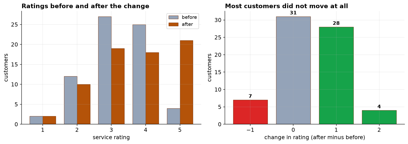
Twenty-eight customers went up by one, four went up by two, and seven went down by one. Nobody moved more than two points, which is the ceiling the instrument imposes.
Why Not a Paired t-test
A paired t-test assumes the differences are approximately normal. Shapiro-Wilk on these differences gives W = 0.848, p = 0.0000006, but the p-value understates the problem. The differences take four distinct values, 44 percent of them identical at zero.
Earlier capstones met skewed data that a log or a square root could tidy up. Nothing does that here, because the problem is not the shape of a continuous distribution. It is the granularity of the measurement. Four possible outcomes will still be four possible outcomes after any transformation you apply to them.
Wilcoxon's signed-rank test ranks the differences by size and compares the rank total for increases against the rank total for decreases. Nothing about equal spacing is assumed, which suits a rating scale exactly.
The Zeros, and the Decision Nobody Mentions
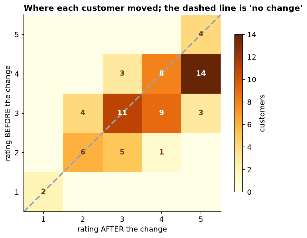
Thirty-one customers changed nothing. A signed-rank test has no natural slot for them: a difference of zero is neither an increase nor a decrease, and it has no size to rank. Every implementation has to decide something, and most do it silently through a default argument.
| Convention | What it does with the zeros | n used | W | p |
|---|---|---|---|---|
| Wilcoxon (1945) | discards them entirely | 39 | 126.0 | 0.000050 |
| Pratt (1959) | ranks them, then drops their ranks | 70 | 343.0 | 0.000048 |
| Split ranks | divides the zero ranks between both sums | 70 | 591.0 | 0.000090 |
They agree here, and that is worth saying plainly. All three land within a factor of two of each other and all three reject the null decisively. This dataset does not force the choice, and it would be dishonest to imply otherwise.
Wilcoxon's original procedure discards the 31 non-movers and tests the 39 who moved, so it answers: among customers whose opinion changed, did it more often improve? Pratt's method keeps them, so it answers: across all customers, did ratings improve? Those are different claims about different populations. With 44 percent of the sample sitting on zero, the second is the one a service manager is asking, which is why it is the one reported here. Whichever you use, state it and state the n it consumed. A reader who sees "n = 39" and a reader who sees "n = 70" are being told about different groups of people.
The Result
Among the 39 customers who moved, the rank total for the 32 improvements is 654 against 126 for the 7 declines. The rank-biserial correlation of 0.68 is that imbalance expressed on a scale from −1 to +1.
The sign test is a useful cross-check. It throws away even the sizes of the changes and looks only at direction, so it assumes less than Wilcoxon does and has less power in exchange. It still rejects at p = 0.00007. When the weakest test available agrees, the conclusion is not resting on an assumption.
Why There Is No Exact p-value
Textbook examples of Wilcoxon usually quote an exact p-value computed by enumerating every possible arrangement of signs. This one cannot, and the reason is structural rather than a matter of software settings.
On a 5-point scale, a change is one point or two points. Across the 39 customers who moved, there are exactly two distinct magnitudes: 35 changes of size 1 and 4 of size 2. The signed-rank procedure ranks by magnitude, so those 35 changes all receive the same average rank, as do the 4.
The exact permutation distribution assumes there are no ties, so it does not apply.
scipy detects the ties, assigns average ranks within each tied block, and switches to the normal
approximation with a tie correction. That is the correct behavior. It is worth recognizing that it happened, rather
than assuming an exact test was simply not requested, because on coarse scales the tie correction is doing real
work.
Statistically Decisive, Practically Modest
The p-value establishes that ratings moved up. It says nothing about whether the movement justifies what the change cost, and those two questions get confused constantly.
| Summary | Value |
|---|---|
| Median rating | 3 before, 4 after: one step on a five-step scale |
| Rated the service higher | 32 of 70 customers (46%) |
| Did not change their answer | 31 of 70 customers (44%) |
| Rated the service lower | 7 of 70 customers (10%) |
| Gave a top-two rating (4 or 5) | 29 before (41%) → 39 after (56%) |
The top-two-box figure, 41 percent rising to 56 percent, is probably the number to put in front of a business, because it corresponds to something an operations team recognizes and it does not require anyone to average an ordinal scale. But the sentence that goes with it should mention the 44 percent who did not move and the 10 percent who moved the wrong way. A statistically decisive result and a modest practical one are perfectly compatible, and this is what that looks like.
What to Watch
- No control group, so no causal claim. The same objection as Capstone 3, and it has not weakened. Ratings could have risen because of the booking change, because of the season, because of a staffing change nobody logged, or because being surveyed twice made customers more forgiving. Without a comparison group that did not receive the change, this shows movement rather than cause.
- Non-response is not random. Three customers never answered the follow-up and were dropped. The people most likely to stop replying are the people who have stopped caring, so the surviving sample probably tilts positive.
- Asking twice changes people. Some customers will answer the second survey partly to be consistent with the first. That pushes differences toward zero, which for once biases against finding an effect rather than toward it.
- Do not report an average rating. Same reasoning as Capstone 12: a mean of an ordinal scale assumes spacing the scale does not provide. Report the distribution or the top-two-box share.
- State the zero convention and the n. Both defensible choices are defensible. Only silence is not.
Paired Rank Tests in Data Science & AI
The before-and-after comparison on the same units is one of the most common shapes in applied work, and the zeros problem travels with it everywhere.
| Where it appears | The paired measurement |
|---|---|
| Model A versus model B on a shared benchmark | The same test items scored under two systems, which is the classic paired setup. |
| Human evaluation of two outputs | The same rater scoring both, on an ordered scale, with plenty of ties. |
| Before and after a deploy | The same users, sessions, or queries measured across a release. |
| Feature-flag rollouts to the same cohort | Each unit acts as its own control, which removes between-user variation. |
Benchmark comparisons between two models are almost always paired, since both are evaluated on the same items, and paired analysis is far more sensitive than treating the two score sets as independent samples. It is also where the zeros problem is most acute: on many benchmarks the two models agree on the majority of items, so the reported n can be a small fraction of the benchmark size. A comparison quoting "p < 0.01" over 800 items, when 760 of them were ties, is describing 40 items. That should be stated, not buried in a default argument.
Estimate: Proportions With Margins
The test established that ratings rose. The operations question is what share of customers moved, and every one of those shares is a proportion estimated from 70 people.
| Quantity | Estimate | 95% CI (Wilson) |
|---|---|---|
| Rated the service higher | 46% | 35% to 57% |
| Did not change their answer | 44% | 33% to 56% |
| Rated the service lower | 10% | 5% to 19% |
| Top-two-box before | 41% | 31% to 53% |
| Top-two-box after | 56% | 44% to 67% |
| Matched-pairs rank-biserial | 0.677 | 0.438 to 0.879 (bootstrap) |
The top-two-box share rose from 41 to 56 percent, and the two intervals overlap heavily. It would be a mistake to conclude from that overlap that the change is unclear, because the same people are measured twice, so the two estimates are not independent. The paired count is the right one: 13 customers moved into the top two boxes and 3 moved out, which on its own terms gives p = 0.02.
That is the same paired-versus-independent distinction the whole chapter rests on, applied to proportions instead of ratings. Treating before and after as two separate samples throws away the pairing and most of the precision it bought.
One more column the analysis had not opened. The file records visits_per_month. Frequent
visitors experience a booking change far more often than occasional ones, so it is a natural place to look for a
difference, and there is not one: visit frequency shows no detectable relationship with how much a rating moved
(ρ = 0.09, p = 0.44), and splitting at the median gives two groups that improved similarly. That is mildly
reassuring, since a change registering only with people who book weekly would be a narrower win than the headline
suggests. It does nothing about the missing control group, because whatever else changed during those months affected
frequent and occasional visitors alike and would leave exactly this trace. Checking a covariate you happen to
have is not the same as having a comparison group.
The full project, step by step
The companion notebook cleans the paired records with a printed audit trail, plots the before-and-after ratings and the distribution of changes, checks the assumption a paired t-test would need and explains why no transformation rescues it, draws the transition matrix that makes the zeros unmissable, then runs all three zero conventions side by side. It computes the effect size, cross-checks with the sign test, shows why the exact test is unavailable, and closes with the practical summary.
The dataset
(capstone-service-ratings-before-after.xlsx) holds the paired ratings with duplicates, follow-up
non-responses, and an impossible rating left in so you can practice the cleaning. Two written reports accompany it:
a plain-language brief for an operations lead, and a technical report covering the
zero conventions, the tie structure, and the effect size.
🎓 Key Takeaways
- ✓Wilcoxon is the paired rank test: it ranks differences by size and compares the rank total for increases against the total for decreases.
- ✓Zeros are a decision, not a detail. Dropping them tests the 39 who moved; keeping them tests all 70. Different questions, different populations, so state which and state the n.
- ✓Coarse scales kill the exact test. With only two distinct change magnitudes, the ranks are heavily tied and the normal approximation with a tie correction is the correct fallback.
- ✓The sign test is the honest cross-check. It assumes almost nothing and still rejected (p = 0.00007), so the conclusion does not depend on the extra assumption Wilcoxon makes.
- ✓Decisive is not the same as large. p = 0.000048, and yet 44% of customers did not move at all and 10% moved the wrong way.
Quiz: Test Yourself
Eight questions on this capstone, from the zeros problem to what a decisive p-value does not tell you. Answer them, hit Check Answers, and keep refining until you score 100%. Your progress is saved.