This is the first capstone where the parametric assumptions fail outright, and the first where the choice of test changes what you may claim, not just how you compute it. Mann-Whitney is usually introduced as the fallback when normality breaks. That undersells it, and this trial shows why.
- Setting
- A trial recorded patient-reported relief on an 11-point numeric rating scale for two treatment arms, New and Standard.
- The question
- Does the new treatment produce more relief than the standard one?
- Why it matters
- A prescribing recommendation follows from the answer, and it has to be stated in something a patient and a prescriber can both act on.
- What we do
- Show why the mean of an ordinal scale has no nameable unit, run the Mann-Whitney test as a comparison of whole distributions, report the probability of superiority and the Hodges-Lehmann shift, and check whether the two arms started level.
The new analgesic beats the standard one decisively (U = 1557.5, p = 0.000028, n = 91). The effect size worth quoting is not a difference in points: pair any new-treatment patient with any standard-treatment patient and the new one does better about three times in four. But the benefit is not spread evenly, and the averages conceal that.
What "Relief" Actually Is
Patients reported relief on an 11-point numeric rating scale, 0 for none and 10 for complete. The number is genuinely ordered: 7 is more relief than 4. It is not a measurement in the way a blood pressure reading is.
If the spacing is not established, then the mean of these scores is a number whose units nobody can name. "The new treatment produced 2.28 more points of average relief" reads like a measurement and is not one. The variable is ordinal and bounded at both ends, which by itself guarantees the data cannot be normal.
Two Very Different Pictures
Cleaning removed two duplicate records, two blanks, and one impossible score of 14 on an 11-point scale, and normalized the treatment labels, leaving 91 patients. Then, before any test, the plot.
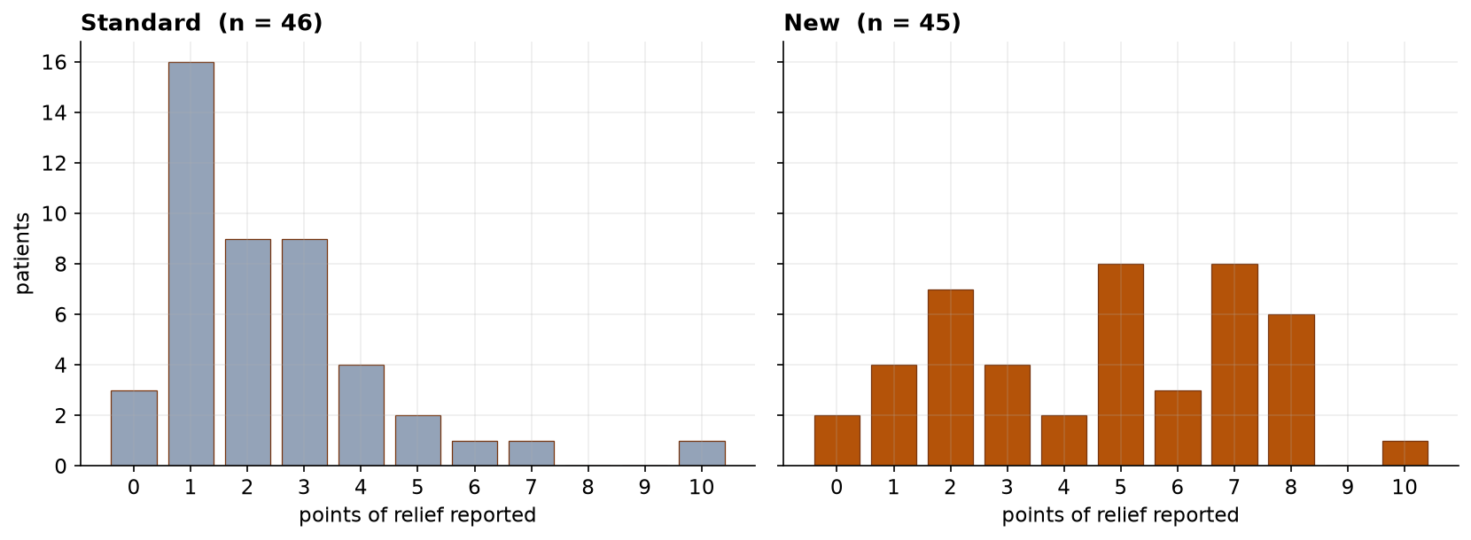
That difference in shape is not a nuisance to be handled. It is the most clinically interesting thing in the dataset, and it comes back in section 6.
The Assumptions, and the Better Reason to Use Ranks
| Check | Standard | New | Verdict |
|---|---|---|---|
| Shapiro-Wilk (normality) | W = 0.830, p < 0.001 | W = 0.941, p = 0.024 | fails in both |
| Skew | +1.71 | −0.09 | strongly right-skewed in one arm |
| Levene (equal spread) | p = 0.006 | fails | |
| Bartlett (equal spread) | p = 0.044 | fails | |
| Standard deviation | 1.94 | 2.63 | 1.36× more variable |
Both parametric assumptions fail. It would be easy to stop there and call that the justification. It is the weaker argument, and here it is nearly beside the point: with 45 patients per arm, a t-test would tolerate this much skew reasonably well, and section 5 shows it reaches the same verdict.
The reason to use ranks is what the outcome is, not what the diagnostics said. A rank test asks a question the scale can answer: are patients on this treatment reporting more relief than patients on that one? That question needs only the ordering, which the scale genuinely provides. A test built on means needs the spacing, which it does not.
The Result
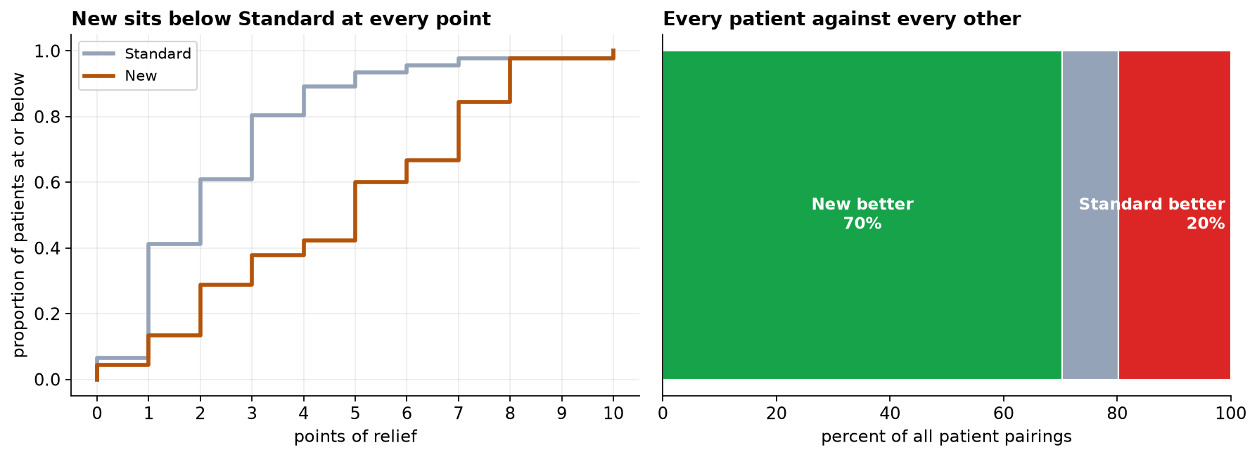
There are 45 × 46 = 2,070 ways to pair one new-treatment patient with one standard-treatment patient. The new patient reported more relief in 70 percent of them and less in 20 percent, with the remaining 10 percent tied. Splitting the ties gives the headline figure: the probability of superiority is 0.75.
It Is Not a Test of Medians
Mann-Whitney is routinely described as "the nonparametric test of medians". That description is wrong, and this trial is exactly the case where being wrong about it matters.
So the defensible sentence for this trial is "in 75 percent of head-to-head pairings the new-treatment patient did better". Writing "the median relief was 3 points higher" would be smuggling in a shift model the data do not support. The medians are 5 and 2, and the difference between them is a real description of these two samples, but it is not what the test established.
The Finding Hiding Under the p-value
A t-test on this data gives t = 4.692, p = 0.000011. It agrees. Nothing here is a case of a parametric test being fooled, and it is worth saying so plainly rather than implying the rank test rescued the analysis. What it did was let us describe the result in terms the measurement supports.
Both tests, though, answer the question that was asked rather than the more useful one. Look at what the summary statistics average over.
| Outcome | Standard (n = 46) | New (n = 45) |
|---|---|---|
| Reported 4 or more points of relief | 9 patients (20%) | 28 patients (62%) |
| Reported almost none (0 or 1) | 19 patients (41%) | 6 patients (13%) |
| Median relief | 2 | 5 |
| Mean relief | 2.39 | 4.67 |
The new treatment does not lift everyone by a couple of points. It splits patients into a group it helps substantially and a group it barely touches. A single summary number, mean or median, describes an average patient who does not appear in this trial. The obvious follow-up is what distinguishes the responders, and that is a question for the baseline data and a fresh study, not for another test on this outcome.
What to Watch, and What Not to Promise
- The outcome is the patient's word. Pain relief is self-reported and cannot be otherwise, since pain is subjective. But that means the measurement carries expectation with it. Without blinding, patients who know they received the new drug may report more relief because they expect more, and this design cannot separate that from a pharmacological effect. The controls argument from Capstone 3 applies here with extra force.
- A responder group is a hypothesis, not a finding. The two clusters are visible and interesting. Hunting through baseline variables for what distinguishes them, and reporting whatever turns up, is the multiple-comparisons trap from Capstone 4 in another costume. Any responder analysis should be pre-specified and confirmed in a fresh trial.
- Do not translate ranks into promises. "Seventy-five percent of pairings favor the new drug" is not "seventy-five percent of patients will be helped". They are different statements, and the second is the one a patient will hear if the first is worded loosely.
- Relief is one column of a wider table. A drug that helps two thirds of patients substantially may still be the wrong choice on side effects, cost, or interactions. This analysis speaks to efficacy on one outcome.
- Ninety-one patients, one recruitment stream. Whether the responder proportion holds in a broader population is unknown from these data.
Rank Tests in Data Science & AI
Bounded, skewed, self-reported outcomes are the norm rather than the exception outside the textbook, and the probability of superiority travels well beyond clinical work.
| Where it appears | Why ranks fit |
|---|---|
| Latency and load-time A/B tests | Response times are hard-floored at zero and heavily right-skewed; the mean is dominated by a long tail. |
| Model output preference studies | Human ratings of two systems on an ordered quality scale, exactly this design. |
| Revenue and engagement per user | A handful of extreme users otherwise drive the entire comparison. |
| Benchmark score comparisons | Bounded metrics that pile up near a ceiling break the equal-spacing assumption. |
The probability of superiority is the effect size to reach for whenever a stakeholder has to act on the result. "Version B is faster for 68 percent of requests" lands where "the mean latency fell by 41 milliseconds" does not, and on a skewed distribution the second number can be driven almost entirely by the tail. The same caution applies as in the trial above: it is a statement about pairings, not about the share of users who will be better off.
Estimate, and Check the Arms Started Level
The headline effect size, a probability of superiority of 0.75, is a point estimate from 91 patients. It deserves an interval as much as any mean does, and the bootstrap supplies one without needing a formula.
| Quantity | Estimate | 95% CI (bootstrap) |
|---|---|---|
| Probability of superiority | 0.752 | 0.648 to 0.845 |
| Rank-biserial correlation | 0.505 | 0.296 to 0.690 |
| Hodges-Lehmann shift | +2.0 points | +1.0 to +4.0 |
| New arm reaching 4+ points relief | 62% | 48% to 75% (Wilson) |
| Standard arm reaching 4+ points | 20% | 11% to 33% (Wilson) |
Even the pessimistic end of the superiority interval is a substantial advantage, which is what makes the finding solid. The honest phrasing for a clinician is "around three times in four, and certainly better than two in three". The responder proportions carry margins too, and they are what a formulary committee will actually use: 62 percent give or take roughly 14 points is what a 45-patient arm can establish.
The file records baseline pain for every patient, which the analysis had not used. In a randomized trial this is the first table of the paper. Here the new-treatment arm started in more pain than the standard arm, 7.31 against 6.70, and the difference is larger than chance comfortably explains (p = 0.011). Randomization balances groups in expectation, not in every particular trial, and with 91 patients a visible imbalance on some variable is far from rare. This is one.
The direction is the unhelpful one. Patients who start in more pain have more room to improve, so an arm that begins worse can look better on a change score for reasons unrelated to the drug. That is regression to the mean, the mechanism that haunted Capstone 3, arriving here through the back door of an unlucky allocation.
Two things stop it overturning the result. Baseline pain barely relates to reported relief in this trial (ρ = 0.08, p = 0.43), so the mechanism that would translate the imbalance into a spurious effect is weak. And the effect itself is large; a 0.6-point head start on an 11-point scale is not going to manufacture a probability of superiority of 0.75. What it changes is the write-up. A trial report that omits this table is hiding something a reader would want. The honest version states the imbalance, states why it is unlikely to explain the finding, and pre-specifies a baseline-adjusted analysis for the confirmatory study. Reporting a randomized trial is not the same as reporting that randomization worked.
The full project, step by step
The companion notebook cleans the trial records with a printed audit trail, plots both distributions before touching a test, runs the normality and equal-spread checks and records what they said, then computes U along with all 2,070 pairwise comparisons behind the effect size. It draws the cumulative curves that make stochastic dominance visible, contrasts a Welch t-test, and closes on the responder split the averages hide.
The dataset (capstone-pain-relief-two-treatments.xlsx) holds
the trial records with duplicates, blanks, an out-of-range score, and inconsistent treatment labels left in so you
can practice the cleaning. Two written reports accompany it: a plain-language brief for a clinical
lead, and a technical report covering the dominance argument, the effect size, and the responder
structure.
🎓 Key Takeaways
- ✓Mann-Whitney tests stochastic dominance, whether one group's values tend to be larger, not whether two medians differ.
- ✓It becomes a test of medians only if the two distributions share a shape. Here one is skewed and one is bimodal, so no single shift exists to report.
- ✓Quote the probability of superiority (0.75): a randomly paired new-treatment patient does better three times in four. It is a claim the ordinal scale supports.
- ✓The stronger case for ranks is measurement, not diagnostics. The t-test agreed (p = 0.000011); what it could not do was report a difference in units anyone can name.
- ✓Look past the summary. 62% of new-treatment patients cleared four points against 20% on standard, but 13% got essentially nothing. The average patient does not exist here.
Quiz: Test Yourself
Eight questions on this capstone, from ordinal measurement to what a rank test may and may not claim. Answer them, hit Check Answers, and keep refining until you score 100%. Your progress is saved.