Capstones 1 and 2 compared separate things: a mean to a target, then two independent groups. This one compares a group to itself. When the same patients are measured before and after a treatment, the two columns are not independent, they are linked person by person, and using that link is the whole point of the paired t-test.
- Setting
- A clinic enrolled hypertensive patients in an eight-week lifestyle-and-medication program and measured each person's systolic blood pressure at the start and at the end.
- The question
- Did systolic blood pressure change over the eight weeks?
- Why it matters
- The clinic is deciding whether to keep funding the program. A drop worth having is one large enough to matter clinically, not merely one small enough to be detected.
- What we do
- Analyze the two readings as pairs with a paired t-test, report the mean change in mmHg with its interval, and then confront what the missing control group does to the conclusion.
Across 55 patients, systolic blood pressure fell about 7 mmHg (146.7 to 139.5). The paired test leaves no doubt, t(54) = 7.37, p < 0.001, with a 95% interval for the drop of [5.3, 9.3] mmHg. The catch, and the real lesson, is that a single before-and-after group cannot prove the program caused it.
The Question, the Hypotheses, the Design
A clinic enrolled hypertensive patients in an eight-week lifestyle-and-medication program and measured each person's systolic blood pressure at the start and at the end. The question is whether blood pressure changed.
| Framework step | This project |
|---|---|
| Goal | Decide whether mean systolic BP changed from before to after the program. |
| Hypotheses | H₀: mean change = 0 vs H₁: mean change ≠ 0, two-sided, α = 0.05. |
| Data type | Two continuous readings per patient (sbp_before, sbp_after), in mmHg. |
| Design | Paired (within-subject): the same people measured twice. Not two independent groups. |
Meet the Data, Then Clean It
The export has 64 rows for 62 patients, and a paired analysis has a strict requirement: a patient is only usable if they have both readings. So the cleaning is: drop duplicate rows, drop patients missing a follow-up (the dropouts), and drop impossible values (a real systolic BP lies between 70 and 250 mmHg, so a 0, a 29, and a 300 all go). That leaves 55 complete pairs.
The right first picture for paired data is a line per patient, from their before value to their after value.
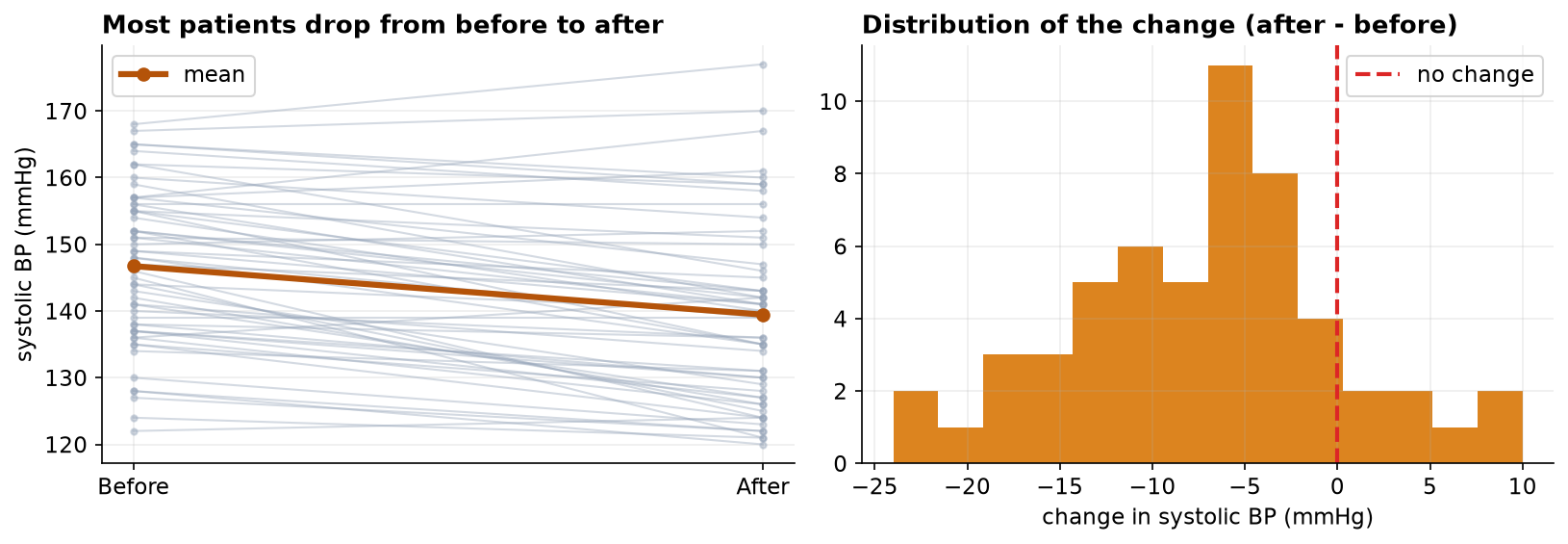
Before averaged 146.7 mmHg, after averaged 139.5, so the mean change is about 7 mmHg down. Whether that drop is real is the question, but first it is worth seeing why the paired design is the strong way to ask it.
Why a Paired Test, and What It Assumes
Patients differ hugely from one another in baseline blood pressure. If we treated the before and after columns as two independent groups, all that person-to-person variation would swamp the eight-week change we care about. Pairing removes it: by taking each patient's own change, the differences between people cancel out, and only the change is left. The paired t-test is then just a one-sample test asking whether those changes average to zero.
Before and after correlate at 0.85 (same people), and using that link shrinks the standard error from 2.44 mmHg (if we wrongly treated the columns as independent) to 0.99 mmHg, about two and a half times more precise. The same data gives a paired t of 7.4 but an independent-samples t of only 3.0. Same numbers, far more power, purely from respecting the design.
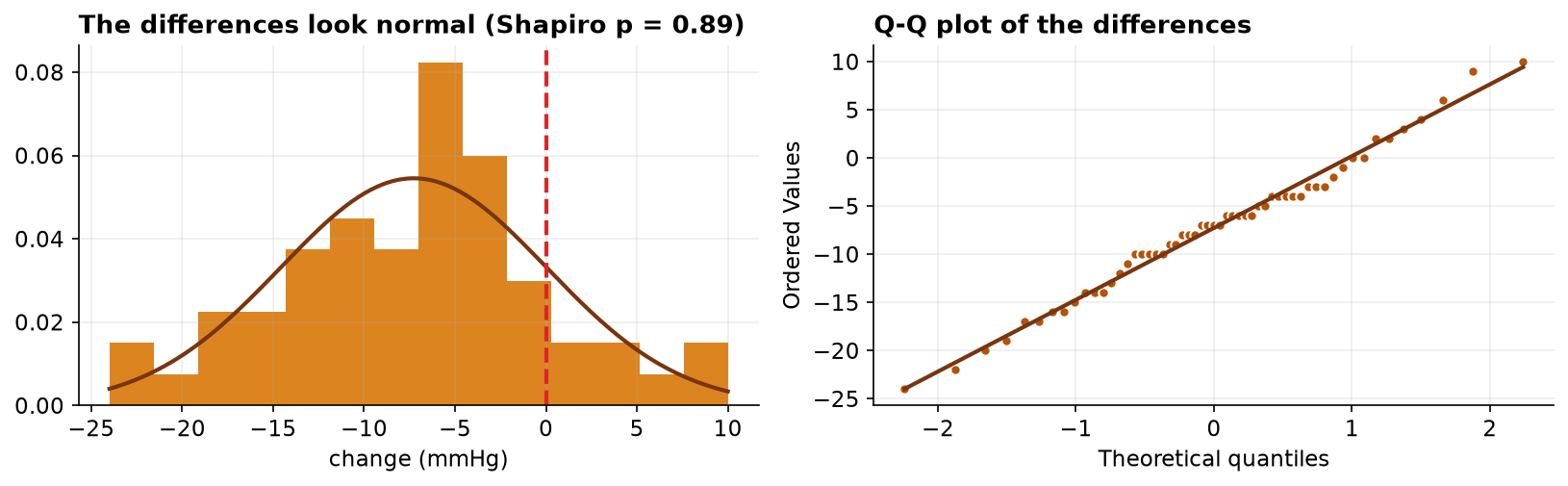
Because the paired test works on the differences, its assumption is about the differences, not the raw readings: the changes should be roughly normal. Shapiro-Wilk gives p = 0.89, and the Q-Q plot agrees, so the assumption holds and no transformation is needed.
Run the Test, Report the Whole Result
The paired t-test asks how far the mean change (about 7 mmHg down) sits from zero, in standard-error units. With the tiny paired standard error, that is more than seven standard errors away, which chance does not produce.
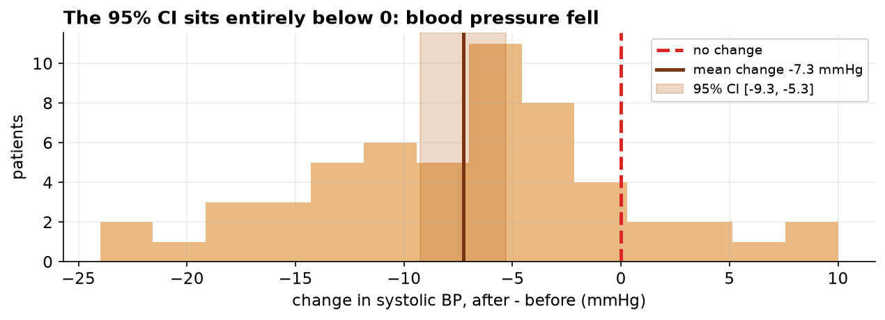
In plain terms: we are 95% confident the true average drop is between 5.3 and 9.3 mmHg, and because that whole range is below zero, blood pressure genuinely fell. The Wilcoxon signed-rank test agrees (p well below 0.001), so the result does not depend on the differences being exactly normal.
The Verdict, and the Missing Control Group
Statistically the answer is settled: blood pressure fell by about 7 mmHg, a large and, clinically, meaningful drop, a sustained 5-to-10 mmHg reduction measurably lowers cardiovascular risk. But the framework's last step is where this project earns its keep, because the honest verdict has a sharp limit.
There was no control group. The paired t-test proves blood pressure changed; it cannot prove the program caused the change, because other explanations fit the same data just as well.
- Regression to the mean. Patients were enrolled because their BP was high. Unusually high readings tend to drift back toward average on their own, with no treatment at all, so some of the drop would have happened anyway.
- Natural change and measurement. Diet, season, a tense first visit (white-coat effect) and a calmer second one can all move blood pressure between two dates.
- Placebo and attention. Being enrolled in a program changes behavior on its own, apart from the program's active ingredients.
- What would fix it. A control group measured the same way but not given the program, ideally randomized, lets you subtract off all of the above and attribute what remains to the program. The paired t-test is the right tool for did it change; it is the wrong tool for did the program cause it.
The Paired t-Test in Data Science & AI
Any time the same units are measured under two conditions, pairing applies, and it appears often in data and ML work.
| Where it appears | The two measurements |
|---|---|
| Model A vs B, same items | Two models scored on the same test examples: compare their per-item errors as pairs. |
| Before / after a change | Latency or accuracy on the same requests, measured before and after a code change. |
| Within-user experiments | Each user tried both variants (a crossover design), so the two readings are paired. |
| Repeated benchmarks | The same benchmark suite run on two configurations of one machine. |
Pairing is the cheapest power boost in statistics: when a comparison can be run on the same units, a paired test often needs a fraction of the sample a between-group test would. The same warning from this chapter applies, though: a before-and-after measurement shows a change but not its cause, so for causal claims you still need a control or a proper experiment.
Estimate, and Ask What Age Was Doing
| Quantity | Estimate | 95% confidence interval |
|---|---|---|
| Change in systolic BP | −7.27 mmHg | −9.25 to −5.29 mmHg |
| Cohen's dz | 0.99 | 0.71 to 1.39 (bootstrap) |
| Before/after correlation | 0.85 | 0.78 to 0.90 (bootstrap) |
A cardiologist asking whether the drop clears a 5 mmHg clinical threshold now gets a straight answer: probably, but the lower end of the interval sits right on it. That is a materially different conversation from "p is less than 0.001". The before-and-after correlation carries an interval too, and it stays high throughout, which is what confirms the pairing is buying real precision rather than getting lucky in this sample.
The file records each participant's age, which the analysis had ignored. Age barely relates to baseline blood pressure here, but it relates to how much blood pressure moved (r = +0.27, p = 0.05). The sign is easy to misread: change is negative, so a positive correlation means older participants dropped less. Split at the median age and the younger half fell 10.2 mmHg against the older half's 4.6, a gap of 5.6 mmHg (p = 0.004) comparable to the whole program effect.
That is effect modification, not confounding. Nothing is explained away; the headline is refined, and the program looks considerably more effective in younger participants. Two cautions come with it. The subgroup split was chosen after seeing the data, which is the trap Capstone 4 is built around, so it is a hypothesis for the next study rather than a finding from this one. And more fundamentally, no covariate you can measure fixes a missing control group: regression to the mean, placebo, and eight weeks of natural variation are not columns in the file, and they would produce an age pattern too.
The full project, step by step
The companion notebook runs all twelve framework steps: it loads the raw file, draws the paired plot, drops the
duplicates, dropouts, and impossible readings with a printed audit trail, checks the normality of the
differences (Shapiro-Wilk, Q-Q), runs the paired t-test with scipy and confirms the effect
size, interval, and power with pingouin, cross-checks with Wilcoxon signed-rank, and shows the
(wrong) independent-samples test to make the value of pairing concrete. Every number here comes from its output.
The dataset (capstone-blood-pressure-before-after.xlsx)
holds the before and after readings on the bp sheet, with a codebook and notes, and it keeps the dropouts,
duplicates, and impossible values so you can practice the paired cleaning. Two written reports accompany it: a
plain-language brief for the clinical lead (result first, with the causation caution), and a
technical report, a journal-style write-up with full methods, the efficiency argument for pairing,
results tables, and references, including a note on what a single-arm design cannot establish.
🎓 Key Takeaways
- ✓The paired t-test is a one-sample test on each subject's change; here systolic BP fell about 7 mmHg over eight weeks.
- ✓Pairing needs both readings: dropouts missing a follow-up cannot be used, so 64 rows became 55 complete pairs.
- ✓Pairing buys power: the before-after correlation (0.85) shrank the standard error 2.5x versus treating the columns as independent.
- ✓Check the differences, not the raw values: Shapiro p = 0.89, so the paired t was valid; t(54) = 7.37, p < 0.001, 95% CI [5.3, 9.3] mmHg, dz = 0.99.
- ✓Change is not cause: with no control group, regression to the mean and other effects could explain part of the drop.
Quiz: Test Yourself
Eight questions on this capstone, from the paired design to the missing control group. Answer them, hit Check Answers, and keep refining until you score 100%. Your progress is saved.