Summary
Prelicensure healthcare students rated ten aspects of their confidence in managing patient aggression immediately before and immediately after an interprofessional high-fidelity simulation, on an eleven-point scale. Of 67 pre-simulation and 72 post-simulation responses, 57 matched on the participant-created identifier.
All ten items improved. Mean differences ranged from 0.70 to 1.74 scale points, with standardized effects from 0.40 to 0.99. Every interval excluded zero, and every item survived Holm correction for ten tests (largest adjusted p = .005). A composite of the ten items rose 1.26 points, 95% CI 0.90 to 1.62, d = 0.95. Because the paired differences are not normally distributed on most items, Wilcoxon signed-rank tests are reported alongside, and agree throughout.
Two problems in the source analysis are documented here. The participant code used to join the two surveys is not unique, so the merged dataset counts some participants more than once; deduplicating leaves every conclusion intact but changes the sample size. Separately, the regression models are reproduced exactly but do not support the interpretation placed on them. See sections 1 and 6.
1. Data and sample construction
Two Qualtrics exports were used, one per survey. Both carry two header rows, the second holding the full question text, so the import reads names from row two and data from row three. Participants are identified only by a code each created from the last two digits of their birth year and their mother's initials. The two files were joined on that code with an inner join, so only participants present in both surveys enter the analysis.
| Stage | n | Note |
|---|---|---|
| Pre-simulation responses | 67 | Complete export |
| Post-simulation responses | 72 | Complete export |
| Matched on participant code | 57 | Analysis set |
| Contributing to a given item test | 53 to 54 | After item-level missingness |
The post survey drew more responses than the pre survey, so the shortfall to 57 is not attrition in the usual sense. It is a matching failure: some participants entered a code that did not reproduce exactly across the two sittings. This matters because a self-created identifier that fails to match is not missing at random in any way the design can verify.
Duplicate participant codes in the merge
The merge is an inner join on a free-text field, and the field is not unique. Three codes appear more than once: one twice in the pre survey and twice in the post survey, two others twice each in the post survey. The duplicated rows carry different answers, in one case comfort ratings of 10 and 7 from the same code before the simulation, so these are different people who happened to construct the same code rather than resubmissions by one person. That is a foreseeable consequence of building an identifier from a birth year and two initials in a cohort of this size.
A SQL inner join on a duplicated key produces every combination of the matching rows. The merged dataset therefore holds 57 rows but only 52 distinct codes, with 5 rows arising from duplication rather than from additional participants. Some responses enter the paired tests two or four times, which inflates n and violates the independence assumption the t-test rests on. Matching is also case-sensitive as written, which costs a further two matches that differ only in capitalization.
Deduplicating on a case-normalized code, keeping the first response per code, gives 54 unique participants. Re-running every comparison on that basis leaves all ten conclusions unchanged. The mean differences are slightly larger and the p-values slightly smaller, because the duplicated rows were pulling toward the null.
| Item | n | Diff. | d | p | n | Diff. | d | p |
|---|---|---|---|---|---|---|---|---|
| Comfort working with an aggressive patient | 54 | 0.70 | 0.46 | .0013 | 51 | 0.78 | 0.52 | .0005 |
| Training for psychological aggression | 54 | 1.17 | 0.70 | <.0001 | 51 | 1.33 | 0.82 | <.0001 |
| Ability to intervene physically | 54 | 0.83 | 0.43 | .0026 | 51 | 0.88 | 0.56 | .0002 |
| Self-assurance in the patient's presence | 53 | 1.15 | 0.66 | <.0001 | 50 | 1.22 | 0.74 | <.0001 |
| Ability to intervene psychologically | 54 | 1.44 | 0.84 | <.0001 | 51 | 1.51 | 0.93 | <.0001 |
| Training for physical aggression | 54 | 1.74 | 0.99 | <.0001 | 51 | 1.80 | 1.06 | <.0001 |
| Feeling safe around an aggressive patient | 54 | 1.61 | 0.69 | <.0001 | 51 | 1.82 | 0.85 | <.0001 |
| Effectiveness of known techniques | 54 | 1.67 | 0.94 | <.0001 | 51 | 1.80 | 1.25 | <.0001 |
| Ability to meet the patient's needs | 54 | 1.46 | 0.83 | <.0001 | 51 | 1.59 | 0.98 | <.0001 |
| Ability to protect yourself physically | 54 | 0.81 | 0.40 | .0045 | 51 | 1.04 | 0.56 | .0002 |
The published result does not change. The reported sample size does. Any restatement of n for this analysis should use the deduplicated figure, and the merge should key on a case-normalized code with duplicates resolved before it is run again.
Is the matched subsample representative?
Comparing pre-simulation composite scores between participants who matched (n = 53, mean 5.32) and those who did not (n = 14, mean 5.01) gives t(20.7) = 0.51, p = .61, using Welch's correction for unequal variances. There is no evidence that the matched subsample started from a different baseline. This is reassurance, not proof: with 14 unmatched cases the comparison has little power to detect a modest difference.
2. The instrument
Ten items, each rated 1 to 11, covering comfort, perceived training for psychological and physical aggression, ability to intervene physically and psychologically, self-assurance, perceived safety, effectiveness of known techniques, ability to meet the patient's needs, and ability to protect oneself. The same ten items were administered at both time points.
Internal consistency is high at both time points: Cronbach's alpha is 0.952 before (n = 57) and 0.983 after (n = 53). Values this high are usually read as good news, and for the purpose of forming a composite score they are. They also indicate redundancy. An alpha above about 0.95 suggests the items are close to measuring one thing, which means the ten tests in section 4 are not ten independent findings. It also weakens the case for reporting ten separate outcomes rather than one composite, and it is the most likely reason the regressions in section 6 behave the way they do.
3. Descriptive statistics
Every item moved upward. The chart below orders items by the size of the change rather than by questionnaire order, which makes the pattern legible: the largest gains are in perceived training and technique, and the smallest are in general comfort and physical self-protection.
| Item | Pre mean | SD | Median | Post mean | SD | Median |
|---|---|---|---|---|---|---|
| Comfort working with an aggressive patient | 6.06 | 2.01 | 6 | 6.76 | 1.84 | 7 |
| Training for psychological aggression | 5.48 | 2.10 | 6 | 6.65 | 1.93 | 7 |
| Ability to intervene physically | 5.63 | 2.59 | 6 | 6.46 | 2.26 | 7 |
| Self-assurance in the patient's presence | 5.49 | 2.26 | 6 | 6.64 | 1.80 | 7 |
| Ability to intervene psychologically | 5.46 | 2.00 | 5 | 6.91 | 1.92 | 7 |
| Training for physical aggression | 4.72 | 2.40 | 5 | 6.46 | 2.17 | 6 |
| Feeling safe around an aggressive patient | 4.83 | 2.40 | 5 | 6.44 | 2.16 | 7 |
| Effectiveness of known techniques | 5.17 | 2.22 | 5 | 6.83 | 1.93 | 7 |
| Ability to meet the patient's needs | 5.28 | 1.91 | 5 | 6.74 | 1.89 | 7 |
| Ability to protect yourself physically | 5.72 | 2.65 | 6 | 6.54 | 2.25 | 6 |
The shift in the comfort item is visible as a compression of the low end rather than a uniform translation. The original document quoted a pre-simulation mean of 5.75 and median 6, rising to 6.58 and median 7. Those figures are computed on the full samples of 67 and 72. Restricted to the 57 matched participants the same item reads 6.06 before and 6.76 after. Both are correct; they answer different questions, and the paired analysis below necessarily uses the matched figures.
4. Primary analysis
Each item was compared within participants using a paired t-test. The quantity of interest is the mean of the post minus pre differences, reported with a 95% confidence interval and with Cohen's d for paired data, defined as the mean difference divided by the standard deviation of the differences. Intervals on d are percentile bootstrap intervals from 5,000 resamples.
| Item | n | Diff. | 95% CI | d | 95% CI | t (df) | p | p Holm |
|---|---|---|---|---|---|---|---|---|
| Comfort working with an aggressive patient | 54 | 0.70 | 0.29 to 1.12 | 0.46 | 0.20 to 0.78 | 3.39 (53) | .0013 | .004 |
| Training for psychological aggression | 54 | 1.17 | 0.71 to 1.62 | 0.70 | 0.40 to 1.08 | 5.17 (53) | <.0001 | <.0001 |
| Ability to intervene physically | 54 | 0.83 | 0.30 to 1.36 | 0.43 | 0.12 to 0.95 | 3.16 (53) | .0026 | .005 |
| Self-assurance in the patient's presence | 53 | 1.15 | 0.67 to 1.63 | 0.66 | 0.35 to 1.11 | 4.79 (52) | <.0001 | <.0001 |
| Ability to intervene psychologically | 54 | 1.44 | 0.97 to 1.91 | 0.84 | 0.53 to 1.27 | 6.16 (53) | <.0001 | <.0001 |
| Training for physical aggression | 54 | 1.74 | 1.26 to 2.22 | 0.99 | 0.73 to 1.34 | 7.26 (53) | <.0001 | <.0001 |
| Feeling safe around an aggressive patient | 54 | 1.61 | 0.97 to 2.25 | 0.69 | 0.38 to 1.18 | 5.07 (53) | <.0001 | <.0001 |
| Effectiveness of known techniques | 54 | 1.67 | 1.18 to 2.15 | 0.94 | 0.54 to 1.55 | 6.92 (53) | <.0001 | <.0001 |
| Ability to meet the patient's needs | 54 | 1.46 | 0.98 to 1.94 | 0.83 | 0.50 to 1.32 | 6.12 (53) | <.0001 | <.0001 |
| Ability to protect yourself physically | 54 | 0.81 | 0.26 to 1.37 | 0.40 | 0.12 to 0.79 | 2.96 (53) | .0045 | .005 |
| Composite of all ten items | 54 | 1.26 | 0.90 to 1.62 | 0.95 | 0.54 to 1.56 | 6.99 (53) | <.0001 | n/a |
The composite score, the mean of a participant's ten items, rose from 5.39 to 6.65, a difference of 1.26 points, 95% CI 0.90 to 1.62, t(53) = 6.99, d = 0.95 with interval 0.54 to 1.56. Given the high internal consistency reported in section 2, this composite is arguably the more defensible primary outcome, and the ten item-level tests are best read as a description of where the change was concentrated.
5. Assumptions and sensitivity
The paired t-test assumes the differences are approximately normal. On 8 of the ten items a Shapiro-Wilk test rejects normality at the 0.05 level. The cause is consistent across items: the differences are left-skewed with heavy tails, because a small number of participants recorded large declines while the bulk clustered on modest gains. The physical-intervention item reaches a change of -8 on an eleven-point scale, with skewness -1.93 and excess kurtosis 7.4. The composite behaves the same way, skewness -1.17 and excess kurtosis 6.0, driven by six participants whose composite did not improve against forty-eight whose did.
| Item | Shapiro-Wilk W | p | Non-normal | Wilcoxon p | t-test p |
|---|---|---|---|---|---|
| Comfort working with an aggressive patient | 0.939 | .0086 | yes | .0034 | .0013 |
| Training for psychological aggression | 0.960 | .0704 | no | <.0001 | <.0001 |
| Ability to intervene physically | 0.841 | <.0001 | yes | .0002 | .0026 |
| Self-assurance in the patient's presence | 0.929 | .0038 | yes | <.0001 | <.0001 |
| Ability to intervene psychologically | 0.945 | .0157 | yes | <.0001 | <.0001 |
| Training for physical aggression | 0.965 | .1134 | no | <.0001 | <.0001 |
| Feeling safe around an aggressive patient | 0.911 | .0007 | yes | <.0001 | <.0001 |
| Effectiveness of known techniques | 0.874 | <.0001 | yes | <.0001 | <.0001 |
| Ability to meet the patient's needs | 0.901 | .0003 | yes | <.0001 | <.0001 |
| Ability to protect yourself physically | 0.902 | .0003 | yes | .0027 | .0045 |
Wilcoxon signed-rank tests, which do not assume normality, reach the same conclusion on every item. The composite behaves the same way: Shapiro-Wilk p = .0004, Wilcoxon p = <.0001. The t-test results are therefore reported as primary with reasonable confidence, since the conclusion does not depend on the assumption that fails.
Multiplicity
Ten tests on ten items inflates the familywise error rate. Holm-Bonferroni adjusted p-values appear in the final column of the table in section 4. All ten items remain significant at the 0.05 level after adjustment, the largest adjusted value being .005. No conclusion here depends on whether or how the correction is applied, which is the useful thing to be able to say.
A note on the original document's summary
The July 2025 summary states that the paired tests produced p-values below .0001 across all ten items. That holds for seven of them. The comfort item (p = .0013), physical intervention (p = .0026), and physical self-protection (p = .0045) are significant but not at that threshold. The corrected values are in the table above and match the SAS output exactly.
6. Regression analysis, and what it does not show
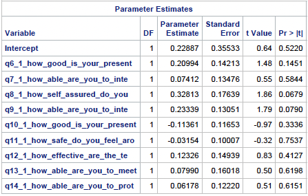
A secondary analysis regressed the comfort item on the other nine items, separately before and after the simulation. The original document reports that the pre-simulation model explains 57.39% of the variance and the post-simulation model 86.77%, and reads the difference as evidence that comfort became more predictable after the simulation.
Both figures reproduce exactly. Refitting from the raw exports gives R² = 0.5739 (n = 67, F = 8.53) and R² = 0.8677 (n = 68, F = 42.27). The numbers are not in question. The interpretation is.
Three problems, in increasing order of severity.
The fit is optimistic. With nine predictors and roughly 67 observations, R² is biased upward. Adjusted R² drops the pre-simulation model to 0.5066. Ten-fold cross-validation, which estimates how the model would perform on data it has not seen, drops it to 0.2247. The honest predictive performance of the pre-simulation model is well under half its reported fit. The post-simulation model holds up considerably better under the same test, at 0.7970.
The predictors are collinear. In the post-simulation model the variance inflation factor reaches 12.4, against a conventional concern threshold of 5 and a serious threshold of 10. This is the direct explanation for the pattern the original document found puzzling: the model is overwhelmingly significant overall, F = 42.27, yet no individual coefficient reaches significance at the 0.05 level. When predictors carry substantially the same information, the model as a whole predicts well while no single coefficient can be estimated precisely. Given a Cronbach's alpha of 0.983, this is expected rather than surprising, and individual coefficients should not be interpreted.
The two R² values are not comparable. They come from different samples (67 and 68 participants), at different points on the response scale, with different amounts of variance available to explain. The sequences of models in the source programs also selected predictors by inspecting collinearity diagnostics on the same data used to report the fit, which biases the reported fit upward by an amount the output does not quantify. A difference in R² between two such models is not evidence about the simulation.
None of this affects the paired comparisons in section 4, which are the study's actual result and which do not depend on any model selection. The regression was described in the original document as an exercise rather than a test of the intervention, and that framing is the right one.
7. Limitations
The design is single-group pre/post with no control condition, so the change cannot be attributed to the simulation alone. Repeating the same ten items within a short window invites both practice effects and demand characteristics, and students who have just completed a training exercise have an obvious reason to report improvement.
The post measurement is immediate, so nothing here speaks to durability. The outcome is self-reported confidence, which is not competence, and the relationship between the two is not established by these data. The identifier-matching shortfall described in section 1 removes about a fifth of respondents from the analysis on grounds unrelated to the intervention. Finally, the ten items are highly intercorrelated, so agreement across all ten is substantially less independent confirmation than it appears.
8. Provenance
Every figure in sections 3 to 5 is computed from the two Qualtrics exports. The paired t-tests were run in SAS on June 27, 2025, and independently reproduced in Python with pandas and SciPy. The two agree on the matched n, the mean difference, and t for all ten items. The regression fits were likewise reproduced to four decimal places. Where this edition adds analyses that were not in the original SAS run, namely the bootstrap intervals on d, the Shapiro-Wilk and Wilcoxon tests, the Holm adjustment, Cronbach's alpha, the selection check, and the cross-validated R², they are computed in Python and identified as such.
Original SAS output
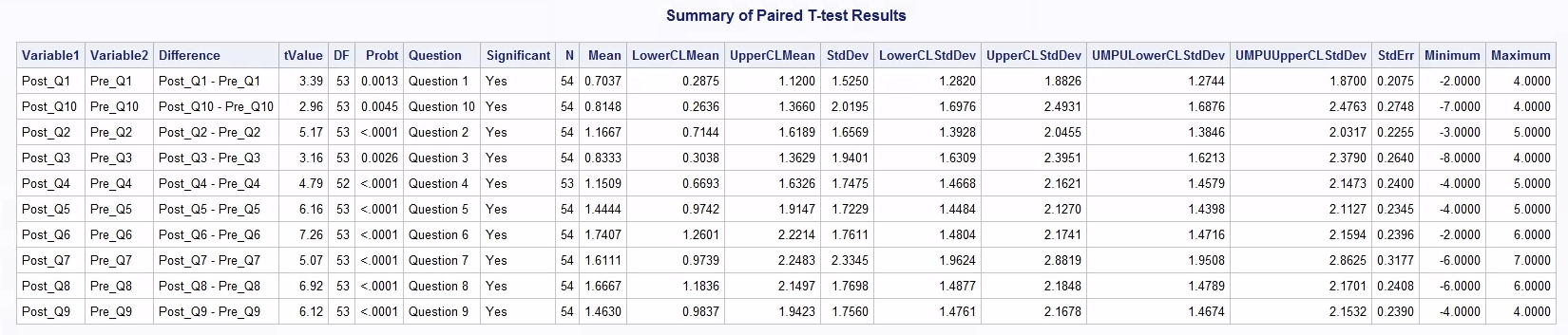
SurveyPairedTTest202506.sas.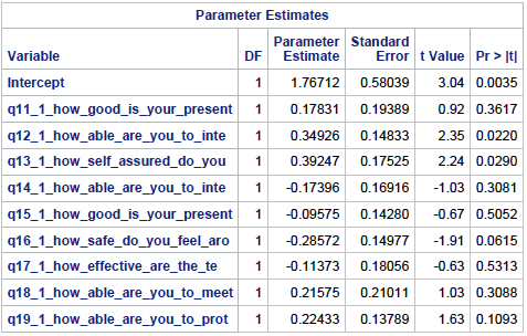
Files
| Artifact | File |
|---|---|
| Paired t-test program | SurveyPairedTTest202506.sas |
| Paired t-test output | 202506_Survey_Paired_TTEST_Results.pdf |
| Pre-simulation program | Survey202506.sas |
| Pre-simulation output | 202506_Survey_Pre_Results.pdf |
| Post-simulation program | SurveyPost202506.sas |
| Post-simulation output | 202506_Survey_Post_Results.pdf |
| Original write-up | Pre and Post Survey Statistical Analysis.docx |
9. What this edition changes
The substance of the July 2025 analysis is unchanged: the simulation is associated with a significant improvement on all ten items, and the paired t-test remains the primary analysis. This edition adds confidence intervals and effect sizes for every comparison, a composite outcome, normality testing with a distribution-free sensitivity analysis, Holm correction for multiplicity, a scale reliability estimate, a check on whether the matched subsample is representative, and cross-validated fit statistics for the regressions.
Two things were corrected. The claim that all ten p-values fall below .0001 is true of seven of them. The reading of the rise in R² from the pre to the post model as evidence about the simulation is not supportable, for the reasons in section 6.