Distribution of Website Traffic Across Days of the Week
A chi-square goodness-of-fit analysis under two competing expected distributions.
Keywords: chi-square goodness-of-fit; expected distribution; Cohen's w; standardized residuals; model specification; drift monitoring.
1. Introduction
The chi-square goodness-of-fit test evaluates whether the observed frequencies of a single categorical variable are consistent with a specified expected distribution. It differs structurally from the test of independence: there the expected counts are derived from the observed marginals, whereas here they are supplied exogenously by the analyst. This distinction is consequential, because the expected distribution is not estimated from the data but asserted, and the test therefore evaluates that assertion as much as the data.
The nominal hypotheses are H₀: the visit distribution equals the specified expectation, against H₁: it does not, with df = k − 1 = 6. This report tests two distinct H₀ specifications to demonstrate the sensitivity of the conclusion to that choice.
2. Data
Data comprise seven aggregated visit totals covering one quarter (N = 3,514). Because the series arrives pre-aggregated, conventional record-level cleaning is inapplicable; validation was limited to confirming seven distinct categories, non-negative integer counts, and no missing values. This is a limitation rather than a convenience: upstream errors such as bot contamination or tracking interruption are not recoverable from aggregates.
| Day | Observed | Expected (uniform) | Standardized residual |
|---|---|---|---|
| Monday | 525 | 502 | +1.03 |
| Tuesday | 569 | 502 | +2.99 |
| Wednesday | 578 | 502 | +3.39 |
| Thursday | 553 | 502 | +2.28 |
| Friday | 510 | 502 | +0.36 |
| Saturday | 406 | 502 | -4.28 |
| Sunday | 373 | 502 | -5.76 |
3. Methods
Pearson's chi-square statistic was computed as the sum of (O − E)²/E across categories, with the expected-count condition (all E ≥ 5) verified prior to testing. Effect size was reported as Cohen's w = sqrt(χ²/N), which is invariant to sample size and therefore separates the magnitude of departure from the power to detect it. Standardized residuals (O − E)/sqrt(E) were inspected to localize discrepancies. The procedure was then repeated with the prior year's empirical shares substituted as the expected distribution. Analyses used SciPy in Python 3.
4. Results
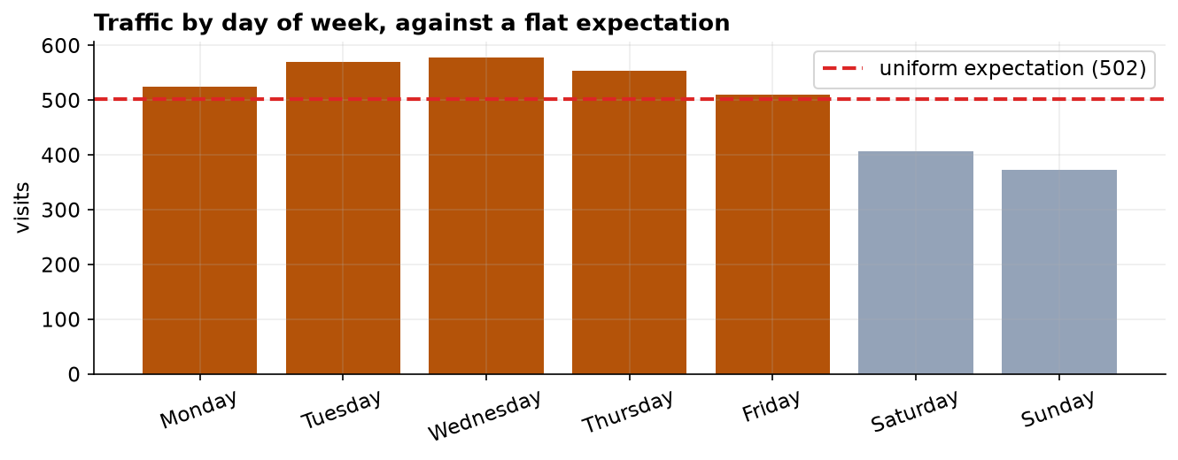
Under the uniform specification the null was rejected decisively, χ²(6) = 78.32, p = 7.95e-15. Standardized residuals localize the departure almost entirely to the weekend, Saturday -4.28 and Sunday -5.76, with midweek days contributing positive but smaller residuals. Cohen's w = 0.149, however, classifies the departure as small; the extreme p-value is substantially a consequence of N = 3,514 rather than of a large discrepancy.
| Expected model | χ²(6) | p | Cohen's w | Decision at α = 0.05 |
|---|---|---|---|---|
| Uniform (1/7 per day) | 78.32 | 7.95e-15 | 0.149 | reject H₀ |
| Prior-year shares | 0.41 | 0.9988 | 0.011 | retain H₀ |
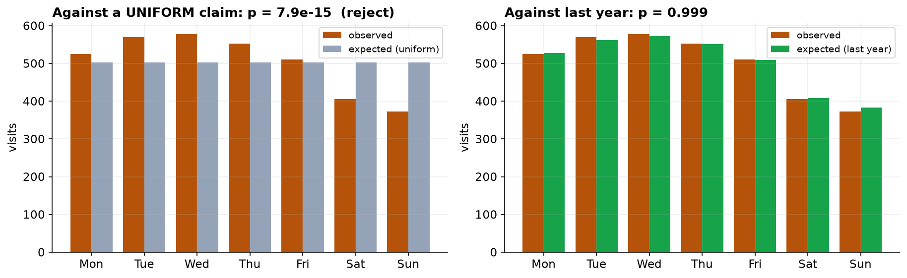
The contrast is the principal result. The observed vector is unchanged between the two analyses; only the reference distribution differs. Under a substantively motivated expectation the data are entirely unremarkable (p = 0.9988, w = 0.011), whereas under an expectation no domain expert would endorse they appear grossly discrepant.
5. Interval estimates by day
| Day | Share | 95% CI | Against 14.29% |
|---|---|---|---|
| Monday | 14.94% | 13.80% to 16.16% | contains |
| Tuesday | 16.19% | 15.01% to 17.45% | above |
| Wednesday | 16.45% | 15.26% to 17.71% | above |
| Thursday | 15.74% | 14.57% to 16.98% | above |
| Friday | 14.51% | 13.39% to 15.72% | contains |
| Saturday | 11.55% | 10.54% to 12.65% | below |
| Sunday | 10.61% | 9.64% to 11.68% | below |
| Cohen's w vs uniform | 0.149 | 0.124 to 0.186 | multinomial resampling |
The omnibus statistic aggregates seven deviations into a single quantity and cannot identify which categories depart from expectation. Interval estimates for the individual shares supply that resolution. Three days lie entirely above an equal allocation and two entirely below, while Monday and Friday cannot be distinguished from it.
The substantive characterization is therefore narrower than the omnibus result implies. The pattern is a midweek elevation and a weekend depression, with the boundary days indeterminate at this sample size. Capacity planning requires the disaggregated estimates rather than the test statistic.
The effect size is bounded between 0.12 and 0.19, lying wholly within the conventional small range. The p-value of 8 × 10⁻¹⁵ quantifies confidence that the departure is not attributable to chance and is frequently misread as quantifying its magnitude; the interval on w precludes that misreading.
6. Discussion
Two defensible conclusions follow from one dataset, and their difference is attributable wholly to model specification. This is not a pathology of the test but a property of it: goodness-of-fit assesses conformity to a stated model, and a rejection is informative only to the extent that the model was a credible candidate. Testing against a straw expectation yields a valid rejection with no inferential content, and because the analyst selects the expectation, this constitutes a researcher degree of freedom that should be removed by pre-specification.
A secondary caution concerns power. With N = 3,514 the test detects departures of negligible practical magnitude; Cohen's w = 0.149 would conventionally be described as small. Reporting the effect size alongside the p-value, and pre-committing to a minimum departure of practical interest, are the appropriate safeguards.
Finally, the prior-year shares are themselves sample estimates carrying sampling error, yet the test treats them as fixed and known. Where the reference distribution is itself estimated, a test accounting for that uncertainty (or a two-sample comparison of the two periods) would be more appropriate than the one-sample form used here.
7. Conclusion
Website traffic is not uniformly distributed across days of the week, χ²(6) = 78.32, p < 0.001, though the departure is small in magnitude (w = 0.149) and confined to the weekend. Against the prior year's pattern the same data show no detectable departure (p = 0.9988). The operationally meaningful conclusion is that the current quarter conforms to precedent; the uniform comparison, though statistically significant, is substantively vacuous.
References
- Pearson, K. (1900). On the criterion that a given system of deviations... Philosophical Magazine, 50(302), 157–175.
- Cochran, W. G. (1952). The χ² test of goodness of fit. Annals of Mathematical Statistics, 23(3), 315–345.
- Cohen, J. (1988). Statistical Power Analysis for the Behavioral Sciences (2nd ed.). Lawrence Erlbaum.
- Agresti, A. (2013). Categorical Data Analysis (3rd ed.). Wiley.
- Simmons, J. P., Nelson, L. D., & Simonsohn, U. (2011). False-positive psychology: undisclosed flexibility in data collection and analysis. Psychological Science, 22(11), 1359–1366.
- Gama, J., et al. (2014). A survey on concept drift adaptation. ACM Computing Surveys, 46(4), 1–37.
Reproducibility
The dataset (capstone-website-visits-by-weekday.xlsx), including the prior-year share sheet, and an executable notebook reproducing every statistic, table, and figure accompany the chapter. Analyses use NumPy, pandas, SciPy, and Matplotlib.