The previous capstone had two categorical variables and asked whether they were related. This one has only one, and asks whether it matches a distribution somebody claimed. That sounds simpler, and mechanically it is. But it hides a trap that the two-variable test does not have: you choose the thing you are testing against, and that choice can manufacture a finding out of nothing.
- Setting
- A company has one quarter of website traffic totaled by day of week, seven counts in all.
- The question
- Is traffic really spread evenly across the week, as marketing has asserted?
- Why it matters
- Staffing, ad scheduling and release timing are all built on the assumption of an even week. If the assumption is wrong, all three are mistimed.
- What we do
- Run a chi-square goodness-of-fit test against the uniform claim, then ask the harder question of whether uniform was ever the right benchmark, and finish by estimating which days differ and by how much.
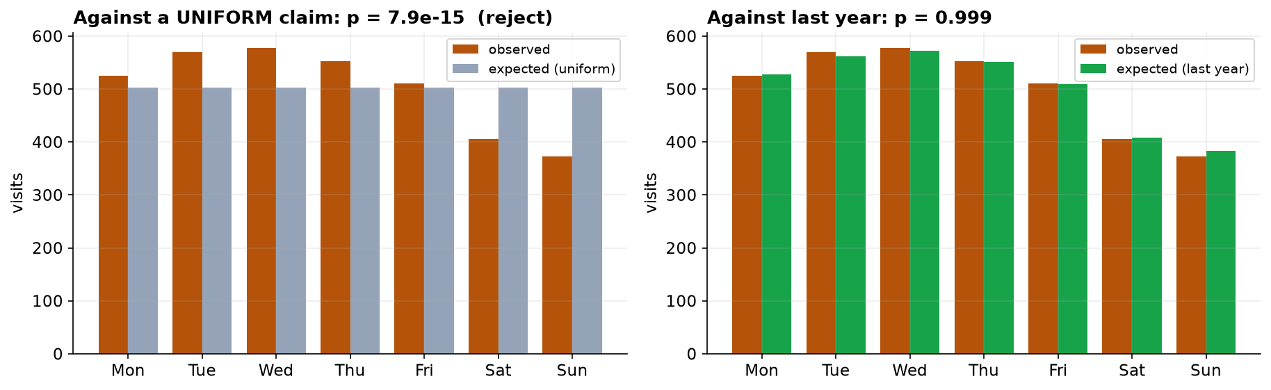
Traffic is emphatically not uniform across the week (χ²(6) = 78.3, p ≈ 8 × 10⁻¹⁵), with weekends far below a flat line. But tested against last year's day-of-week pattern the very same numbers give p = 0.999. Same data, opposite verdicts. The expected distribution is the hypothesis.
One Variable, One Claim
A company has a quarter of website traffic totaled by day of week, and someone in marketing has asserted that traffic is spread evenly across the week. The data are seven counts, and the assertion is a distribution.
That difference is the whole point. In a test of independence the expected counts come from the table itself. In a goodness-of-fit test you bring the expected distribution with you, which means you are testing your own assumption as much as the data.
The Obvious Test, and Its Obvious Answer
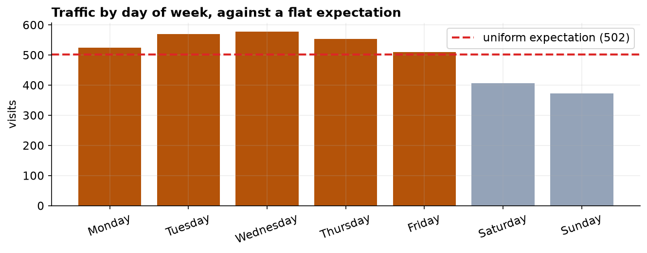
With 3,514 visits over seven days, a uniform claim expects about 502 per day. Every expected count is far above the minimum of 5, so the approximation is safe.
| Day | Observed | Expected (uniform) | Standardized residual |
|---|---|---|---|
| Monday | 525 | 502 | +1.03 |
| Tuesday | 569 | 502 | +2.99 |
| Wednesday | 578 | 502 | +3.39 |
| Thursday | 553 | 502 | +2.28 |
| Friday | 510 | 502 | +0.36 |
| Saturday | 406 | 502 | −4.28 |
| Sunday | 373 | 502 | −5.76 |
Note the tension already visible in those four numbers. The p-value is astronomically small, and the effect size is small. With 3,514 visits the test can detect a modest departure easily, so the p-value is reporting the sample size as much as the size of the pattern.
But Was Uniform Ever the Right Claim?
Here is the trap. We rejected "traffic is uniform", but nobody who runs a website expects uniform traffic. Weekends are quieter for most business sites. Rejecting a claim no one believed is a technically valid result that carries no information, and it is one of the easiest ways to manufacture a finding.
So test a claim someone would actually make: that this quarter matches last year's day-of-week shares, which already build in the weekend dip.
| Expected model | χ²(6) | p | Cohen's w | Verdict |
|---|---|---|---|---|
| Uniform (one seventh per day) | 78.32 | 8 × 10⁻¹⁵ | 0.149 | reject |
| Last year's day-of-week shares | 0.41 | 0.999 | 0.011 | do not reject |
A goodness-of-fit test does not tell you whether data are "normal" or "fine". It tells you whether they match the specific distribution you handed it. A rejection means the data disagree with that model, and the value of the result depends entirely on whether the model was worth testing. State and justify the expected distribution before running the test, or the test becomes a formality wrapped around a foregone conclusion.
The Verdict
Both statements below are true, and only one is worth putting in a report:
- "Traffic is not evenly spread across the week." Correct, highly significant, and of no use to anyone. It rejects an expectation nobody held.
- "Traffic this quarter is indistinguishable from last year's pattern." Also correct, and actually informative: there is no anomaly to investigate and no change to explain.
The honest one-line summary is that traffic is uneven across the week in exactly the way it always has been. Weekdays run about a fifth above the weekend, Sunday is the quietest day, and nothing this quarter departs from precedent.
Ethics, Bias, and Limits
- Choosing the null is an ethical act. Picking an expected distribution nobody believes, then rejecting it, produces a headline with no content. Because the analyst controls that choice, it must be declared and defended in advance rather than selected after seeing which one "works".
- Large samples make small departures significant. Cohen's w of 0.15 is small; the tiny p-value comes largely from 3,514 visits. Decide beforehand what size of departure would actually change a decision.
- Aggregated data cannot be audited. Seven totals cannot reveal a bot surge on one afternoon, a tracking outage, or a misattributed redirect. Pre-aggregation removes exactly the detail that cleaning would catch, so provenance matters more here, not less.
- The comparison model carries its own uncertainty. Last year's shares are themselves estimates, but the test treats them as exact. And a quarter is a season: holidays, campaigns, and school terms shift the pattern, so this quarter's shape may not transfer to the next.
Goodness-of-Fit in Data Science & AI
Comparing an observed distribution against an expected one is a routine production task, usually under a different name.
| Where it appears | The expected distribution |
|---|---|
| Data-drift monitoring | This week's category mix against the training-set mix. |
| A/B assignment checks | Observed split across arms against the intended 50/50 or 33/33/33. |
| Survey weighting | Sample demographics against known census shares, before raking. |
| Fraud and anomaly screens | Observed leading digits against Benford's law. |
Drift monitors are where this test most often goes wrong in production. At scale every distribution differs from its reference, so a chi-square alarm fires constantly and gets ignored, which is worse than no alarm. The fix is the discipline from this chapter: choose a reference distribution that reflects genuine expectation, alert on an effect size threshold rather than a p-value, and pre-commit to how large a shift has to be before anyone should care.
Estimate: Which Days, and by How Much
Two chi-square tests gave two verdicts. Neither said how far any particular day sits from its expectation, and that is the only form in which this result reaches a planning meeting. A Wilson interval on each day's share does the job the omnibus test cannot.
| Day | Visits | Share | 95% CI (Wilson) | Against an even split (14.29%) |
|---|---|---|---|---|
| Monday | 525 | 14.94% | 13.80% to 16.16% | contains 14.29% |
| Tuesday | 569 | 16.19% | 15.01% to 17.45% | above |
| Wednesday | 578 | 16.45% | 15.26% to 17.71% | above |
| Thursday | 553 | 15.74% | 14.57% to 16.98% | above |
| Friday | 510 | 14.51% | 13.39% to 15.72% | contains 14.29% |
| Saturday | 406 | 11.55% | 10.54% to 12.65% | below |
| Sunday | 373 | 10.61% | 9.64% to 11.68% | below |
Only three days sit entirely above an even share, and two sit entirely below. Monday and Friday are on the fence: both intervals contain 14.29 percent, so the two ends of the working week cannot be distinguished from an even split this quarter. The omnibus test could never have told us that, because it collapses seven deviations into one number. If capacity planning is the goal, this table is the output and the p-value is not.
The effect size gets an interval too. Cohen's w against the uniform expectation is 0.149, with a 95 percent interval of roughly 0.12 to 0.19. The whole of that range sits in "small" territory. This matters for how the result is sold: traffic is not evenly spread and the departure is real, but it is not dramatic. A p-value of 8 × 10⁻¹⁵ describes how confident we are that the pattern is not chance, and it is routinely misread as describing how big the pattern is.
The full project, step by step
The companion notebook runs the framework end to end on aggregated data: it validates the seven categories,
checks the expected counts, runs the goodness-of-fit test against the uniform claim with scipy,
computes Cohen's w and the standardized residuals, then re-runs the identical test against last year's shares
and plots the two comparisons side by side. Every number here comes from its output, with a plain-language note
after each result.
The dataset (capstone-website-visits-by-weekday.xlsx) holds
the seven daily totals on the visits sheet and last year's shares on the PriorYear sheet, so you
can run both tests yourself. Two written reports accompany it: a plain-language brief for a
marketing lead, and a technical report with both models, residuals, effect sizes, and references.
🎓 Key Takeaways
- ✓Goodness-of-fit tests one variable against an expected distribution, with df = k − 1. Independence tests two variables and derives its expectation from the table.
- ✓You supply the expected distribution, so it is a hypothesis, not a fact. Declare and justify it before testing.
- ✓Same data, opposite verdicts: uniform gave χ²(6) = 78.3, p ≈ 8 × 10⁻¹⁵; last year's shares gave χ²(6) = 0.41, p = 0.999.
- ✓Report the effect size: Cohen's w of 0.15 is small, and the vanishing p-value mostly reflects 3,514 visits.
- ✓Rejecting a claim nobody held is not a finding. "Traffic is uneven" was true and useless; "traffic matches last year" was the informative answer.
Quiz: Test Yourself
Eight questions on this capstone, from degrees of freedom to choosing the null. Answer them, hit Check Answers, and keep refining until you score 100%. Your progress is saved.