Association Between Self-Reported Study Hours and Examination Performance
Pearson correlation with influence diagnostics and a rank-based comparison.
Keywords: Pearson correlation; Fisher z interval; influential observations; Spearman's rho; measurement error; causal inference.
1. Introduction
Correlation quantifies the strength and direction of linear co-variation between two continuous variables. Its principal virtue, reduction to a single interpretable coefficient, is also its principal hazard: markedly different bivariate structures can yield identical coefficients, and the statistic is not resistant to observations with high leverage. Graphical inspection prior to estimation is therefore not stylistic preference but methodological requirement.
The hypotheses are H₀: ρ = 0 against H₁: ρ ≠ 0, evaluated two-sided at α = 0.05. The analysis additionally specifies an influence assessment in advance, so that the reported coefficient is accompanied by a statement of its stability rather than presented as a point estimate of unexamined robustness.
2. Data
Records comprise a student identifier, self-reported weekly study hours, and final examination score bounded 0 to 100. Cleaning removed one duplicate record, two records with a missing outcome, and one record reporting negative study hours, yielding n = 90.
| Step | Rule | Result |
|---|---|---|
| Raw export | — | 94 rows |
| De-duplication | drop duplicate rows | 93 rows |
| Missing values | drop rows missing either variable | 91 rows |
| Range filter | retain study hours > 0 | 90 rows |
| Variable | Mean | SD | Min | Max | Shapiro-Wilk p |
|---|---|---|---|---|---|
| Study hours / week | 11.14 | 3.46 | 1.9 | 21.5 | 0.282 |
| Exam score | 74.14 | 10.72 | 38 | 99 | 0.139 |
3. Methods
The bivariate scatterplot was inspected before estimation to assess linearity and identify potentially influential observations. Pearson's r was computed, with a confidence interval obtained via the Fisher z transformation, z = arctanh(r), with standard error 1/sqrt(n − 3), back-transformed to the correlation scale. Influence was quantified by leave-one-out refitting for the observation with the largest absolute residual from the least-squares line. Spearman's rank correlation was computed as a robustness comparison, since rank-based statistics are resistant to extreme values in either margin. Analyses used SciPy in Python 3.
4. Results
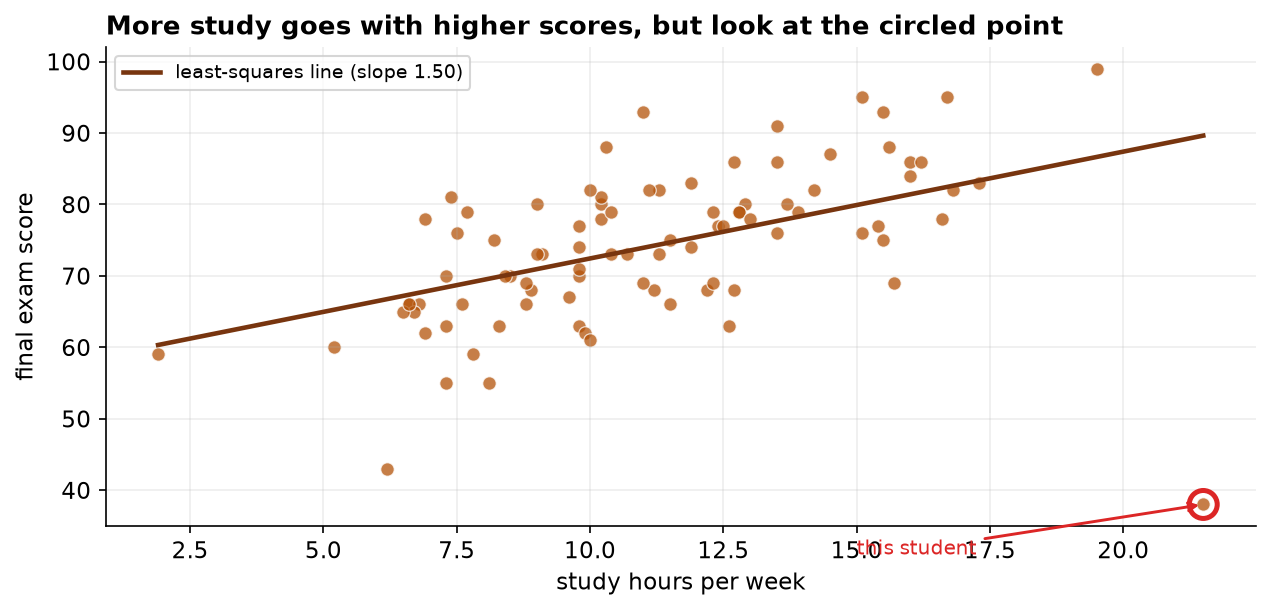
The relationship is approximately linear with no evident curvature, supporting the use of a product-moment coefficient. One observation is visually discrepant, combining high exposure with a low outcome.
| Statistic | Value | Interpretation |
|---|---|---|
| Pearson r | 0.483 | moderate positive association |
| p-value | 1.40e-06 | reject H₀: ρ = 0 |
| 95% CI (Fisher z) | [0.307, 0.628] | excludes zero |
| r² | 0.234 | approx. 23% of outcome variance accounted for |
| n | 90 | complete cases |
| Specification | Coefficient | Change from primary |
|---|---|---|
| Pearson r, all observations | 0.483 | — (reported) |
| Pearson r, leave-one-out | 0.676 | +0.193 |
| Spearman ρ, all observations | 0.613 | +0.130 |
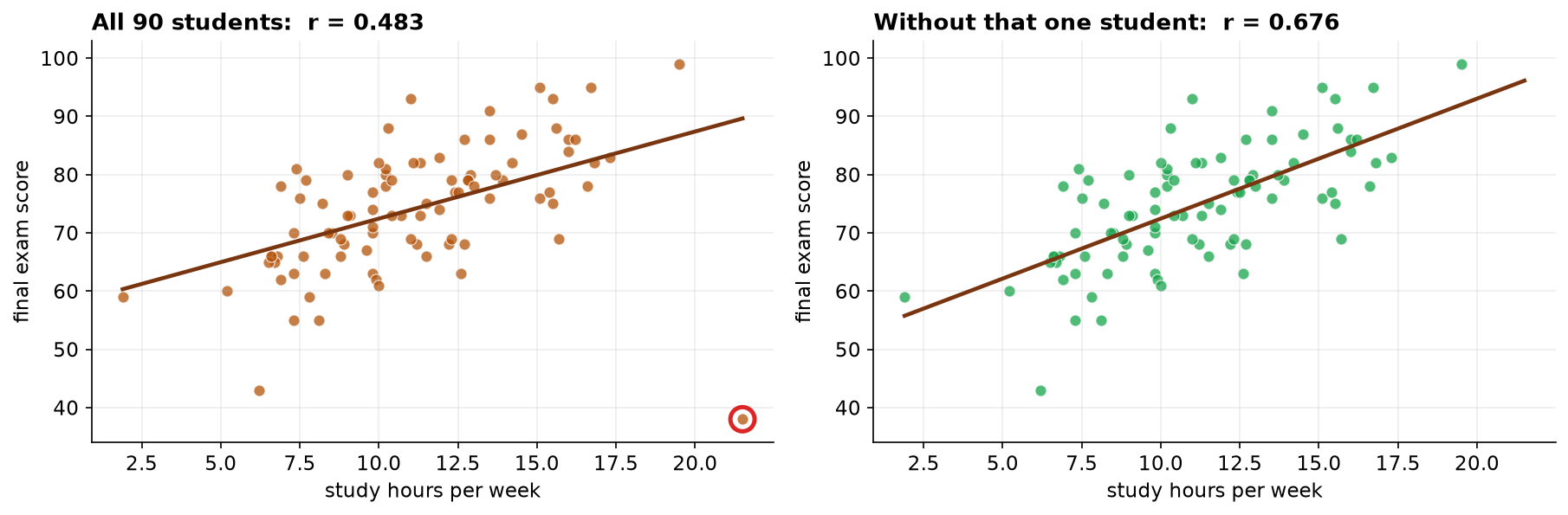
The leave-one-out shift of +0.193 is substantial for a single observation in a sample of 90, moving the descriptive characterization from moderate to strong. Spearman's ρ = 0.613 lies nearer the leave-one-out estimate, which is diagnostic: the observation is extreme in the outcome margin relative to its exposure, so it exerts leverage on the product-moment statistic while affecting ranks only marginally. The observation is retained, being a valid measurement rather than a recording error, and its influence is disclosed.
5. Covariance, and two disagreeing intervals
| Quantity | Estimate | 95% CI | Method |
|---|---|---|---|
| Pearson r | 0.483 | 0.307 to 0.628 | Fisher z transformation |
| Pearson r | 0.483 | 0.126 to 0.750 | percentile bootstrap |
| r² | 0.234 | 0.016 to 0.563 | percentile bootstrap |
| Spearman ρ | 0.613 | 0.433 to 0.754 | percentile bootstrap |
| Pearson r, observation excluded | 0.676 | 0.555 to 0.773 | percentile bootstrap |
The product-moment coefficient is a normalization of the covariance by the product of the marginal standard deviations. The covariance for these data is 17.9 in units of hours multiplied by marks, a quantity without interpretable scale: recording exposure in minutes multiplies it sixtyfold and rescaling the outcome multiplies it again, while the correlation is invariant at 0.483 throughout. The invariance is the purpose of the normalization, and it is also the reason the coefficient is bounded by unity, the covariance being unable to exceed the product of the standard deviations.
The two interval constructions do not agree, and the discrepancy is diagnostic. The Fisher transformation assumes bivariate normality and is not resistant to high-leverage observations; the sample contains one. The bootstrap interval is approximately twice the width. Where a parametric interval and a resampling interval diverge materially, the divergence generally indicates that a distributional assumption is not satisfied, and the resampling interval is the appropriate one to report.
The consequence for interpretation is substantial. The proportion of outcome variance associated with exposure is bounded between approximately 2 and 56 percent. A point estimate of 23.4 percent implies a precision the design does not support.
6. Discussion
A moderate positive association between study hours and examination performance is established, accounting for approximately 23% of outcome variance. The complement of that figure is the more important communication point: the majority of between-student variation is attributable to factors this survey did not measure.
Three limitations constrain interpretation. First, the design is cross-sectional and observational, so the correlation is compatible with at least three causal structures: exposure causing outcome, reverse causation (facility with the material rendering study more tractable and simultaneously producing higher scores), and confounding by a common antecedent such as prior achievement or motivation. These are not distinguishable by any increase in sample size; they are distinguishable only by design.
Second, the exposure is self-reported. Systematic over-reporting of study time, plausibly differential by attainment, constitutes measurement error in the predictor, which attenuates the observed coefficient toward zero. The true association may therefore exceed the estimate reported here. Third, range restriction applies: the sample comprises students who enrolled and sat the examination, and the association may differ in a population including non-completers.
Finally, the sensitivity of r to a single observation argues against reporting the coefficient to a precision the data do not support, and in favor of reporting the interval together with the leave-one-out estimate, as done here.
7. Conclusion
Self-reported weekly study hours and final examination score are positively associated, r = 0.483 (95% CI [0.307, 0.628], p < 0.001), with r² = 0.234. The estimate is sensitive to one influential observation (leave-one-out r = 0.676), which is retained and disclosed. The design does not support causal interpretation, and self-reported exposure likely attenuates the estimate.
References
- Pearson, K. (1896). Mathematical contributions to the theory of evolution III: regression, heredity and panmixia. Phil. Trans. R. Soc. A, 187, 253–318.
- Fisher, R. A. (1915). Frequency distribution of the values of the correlation coefficient in samples from an indefinitely large population. Biometrika, 10(4), 507–521.
- Anscombe, F. J. (1973). Graphs in statistical analysis. The American Statistician, 27(1), 17–21.
- Cook, R. D. (1977). Detection of influential observation in linear regression. Technometrics, 19(1), 15–18.
- Spearman, C. (1904). The proof and measurement of association between two things. American Journal of Psychology, 15(1), 72–101.
- Carroll, R. J., Ruppert, D., Stefanski, L. A., & Crainiceanu, C. M. (2006). Measurement Error in Nonlinear Models (2nd ed.). Chapman & Hall.
Reproducibility
The dataset (capstone-study-hours-and-scores.xlsx) and an executable notebook reproducing every statistic, table, and figure accompany the chapter. Analyses use NumPy, pandas, SciPy, and Matplotlib.