The trading team has twenty weeks of prices and sales and would like to know what a pricing agent would have earned on it. The answer is that twenty weeks of history cannot say, and finding out why is most of the work.
- Setting
- An online retailer with 40 products. Two logs: 140 days of business as usual, where price was a cost-plus markup by category with a sitewide sale every fifth week, and 84 days of a randomized price experiment run afterwards with the assignment probabilities recorded.
- The question
- Should the site replace its cost-plus rule with an agent that sets prices day by day, and what would that agent be worth?
- Why it matters
- A pricing agent acts on every customer, every day, and it will exploit any error in the model it was trained on. Getting this wrong is not a bad forecast, it is a wrong price on the whole catalog.
- What we do
- Show that the historical log cannot identify the price effect, show what the experiment bought and why its design mattered, build a simulator, compare a myopic agent against a far-sighted one against a Q-learner, price exploration, and measure how much the simulator's errors cost.
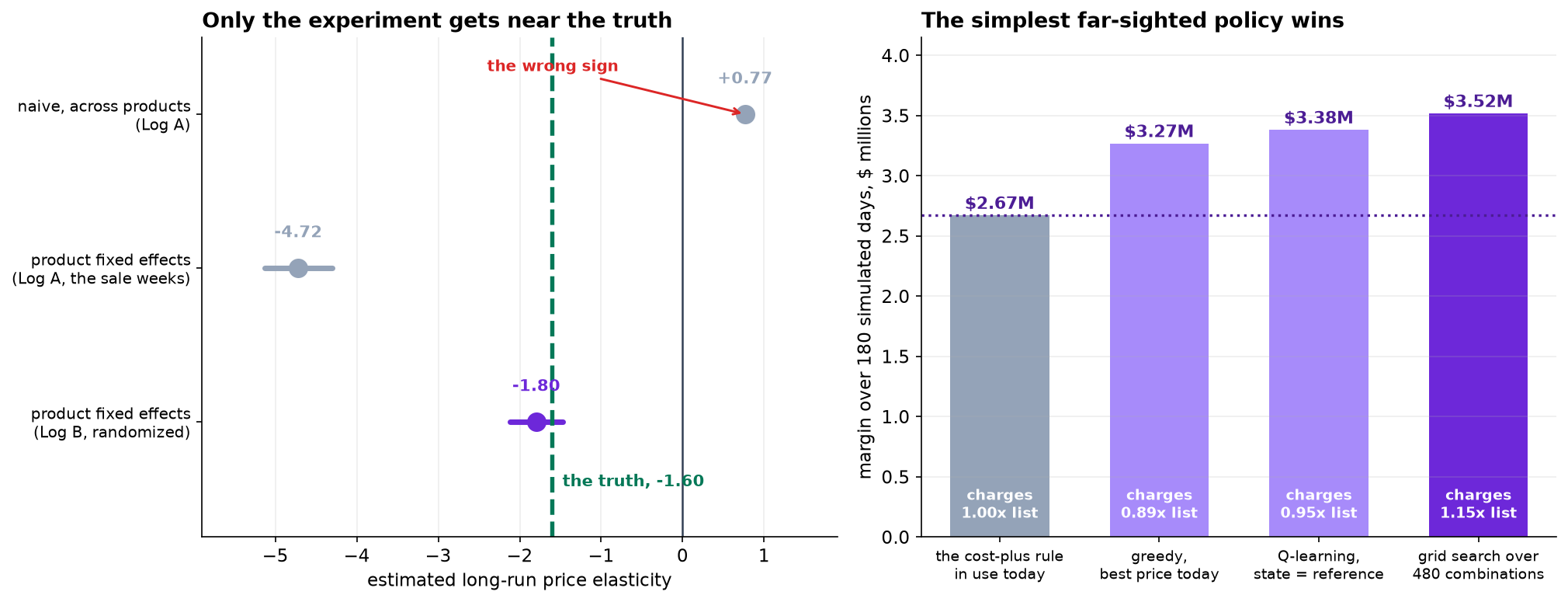
The obvious regression on twenty weeks of history says the price coefficient is +0.77: raising prices raises demand. Product fixed effects fix the sign and put it at −4.72 against a truth of −1.60. Only the randomized experiment gets close. And when the agents are compared, the Q-learner loses to a grid search over 480 combinations, for a reason visible in the policy it learned.
The Regression the Team Already Ran
The first number is not a small effect or a marginal result. It is firmly estimated, tightly bounded and completely wrong, and the reason is in the product table: the dearer products cost more to make, and they are better. Price was never an experiment run on customers, it was a markup applied to a catalog, so a comparison across products is a comparison between different products rather than between different prices for the same one.
The repair looks obvious. Compare a product against itself, with product fixed effects. That fixes the sign and does not fix the number.
After the fixed effects there is almost no price variation left. The only time a product's price moves is the sitewide sale every fifth week, and the sale never arrives on its own: it comes with the email blast and the homepage banner. The one price change in the dataset is perfectly confounded with a demand shock, so the model attributes the whole of the promotional lift to the price cut and reports an elasticity nearly three times too large.
A fixed effect removes a confounder between units. It cannot manufacture variation that was never there.
What the Experiment Bought
Six weeks of randomization changes both things that were wrong.
| Log A, business as usual | Log B, randomized | |
|---|---|---|
| Price multipliers ever shown | 2 of 7 | 7 of 7 |
| Assignment probability recorded | no | yes |
| Spread of reference price around list | 0.024 | 0.049 |
| Long-run elasticity | −4.72 | −1.80 [−2.12, −1.47] |
| Short-run elasticity | −2.06 | −2.10 [−2.47, −1.74] |
Truth: long run −1.60, short run −2.46. Both estimates are mildly attenuated because the logs aggregate sessions to product-days, and averaging inside a logit shrinks a coefficient toward zero.
Two design choices in that experiment did the work, and both are easy to get wrong.
The prices were held for a week at a time. Daily re-randomization would have identified the total price response and would not have separated the short-run effect from the long-run one, because the reference price never moves if the price bounces around a constant average. Separating them requires the thing customers anchor on to actually drift, and that takes weeks.
The assignment probability was written down. That column is what makes offline evaluation possible at all, and it is the one most often thrown away as an implementation detail.
Estimating a Policy Before Deploying It
To estimate what a new policy would have earned from data generated by an old one, reweight each logged outcome by how likely the new policy was to take the action that was taken, divided by how likely the old one was. Under the cost-plus rule that denominator is zero for five of the seven prices, so the estimate does not exist. On the randomized log it does.
The estimate is unbiased and the interval is wide, and both come from the same place. A policy that always charges 1.10 only learns from the tenth of the log where 1.10 was assigned, so evaluating a deterministic policy offline discards most of the data by construction. That is the honest price of not deploying it, and it is a good argument for keeping a slice of randomization running permanently.
The Promotion Trap
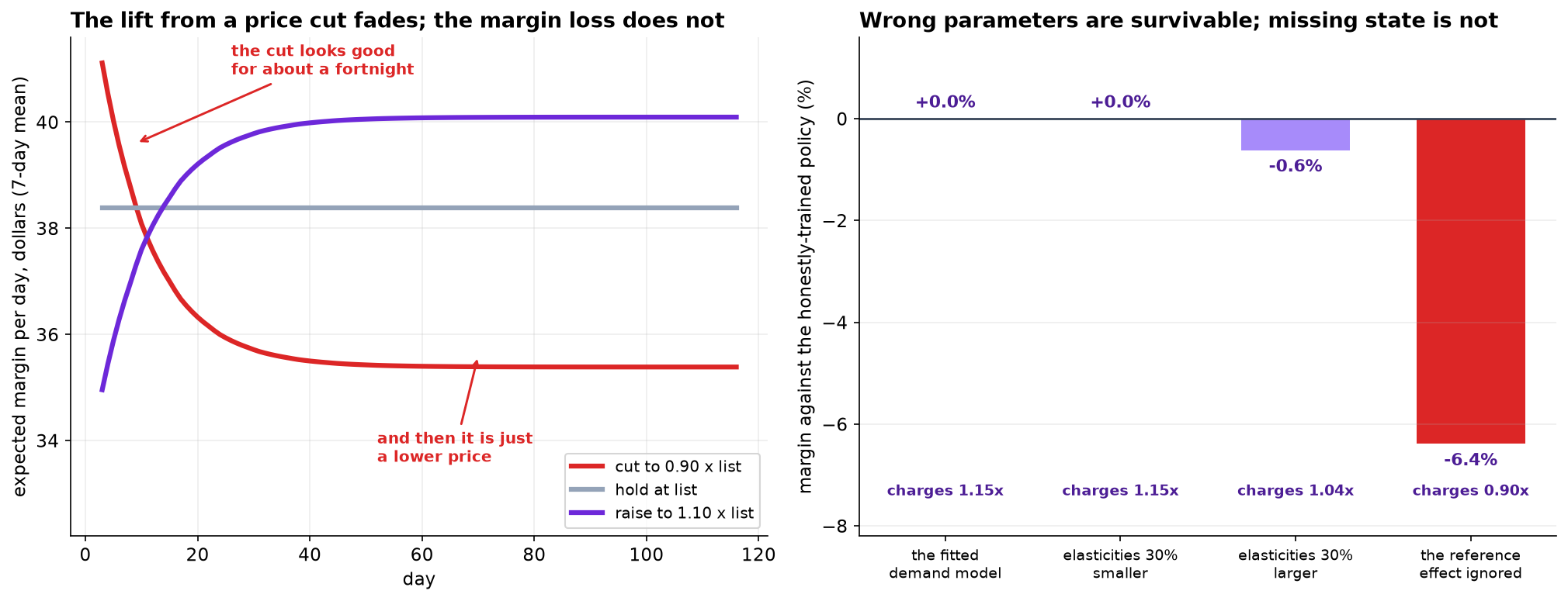
The estimated demand model has two price terms, and the difference between them is the whole reason this is a sequential problem rather than a bandit. A cut buys the short-run response of about −2.1, because customers compare today's price with what they expected. Hold the cut and the expectation follows it down over a few weeks, leaving only the long-run response of about −1.8 against a permanently lower price.
| Policy | Margin, 180 days | Against the rule | Charges |
|---|---|---|---|
| The cost-plus rule in use today | $2,670,341 | — | 1.00× list |
| Greedy, best price for today | $3,266,629 | +22.3% | 0.89× list |
| One fixed price, best over the horizon | $3,516,368 | +31.7% | 1.15× list |
The greedy agent cuts prices about ten percent and the far-sighted one raises them about fifteen, and the far-sighted one earns 7.6 percent more. A myopic optimizer sees only the larger of the two elasticities, so it discounts. The mistake is not in the optimization. It is in the horizon.
The Reinforcement Learner, and Why It Lost
A fixed price cannot respond to circumstances. A Q-learner can: state is where the reference price sits relative to list, action is one of seven multipliers, reward is the day's margin.
| Discount factor | Effective horizon | Margin | Against the rule | Charges |
|---|---|---|---|---|
| 0.90 | 10 days | $3,380,090 | +26.6% | 0.95× list |
| 0.97 | 33 days | $3,068,521 | +14.9% | 0.96× list |
| 0.995 | 200 days | $3,045,479 | +14.0% | 0.96× list |
| 0.999 | 1000 days | $2,960,571 | +10.9% | 0.92× list |
Every one of them loses to the grid search, and a longer horizon makes it worse rather than better. That is worth diagnosing rather than tuning away, so look at what the agent learned.
| Where the reference price sits | What the agent charges |
|---|---|
| Below 0.90 × list | 1.015 × list |
| 0.90 to 0.96 | 0.974 |
| 0.96 to 1.02 | 0.965 |
| 1.02 to 1.08 | 0.906 |
| Above 1.08 | 0.896 |
The agent has learned to chase the reference price. When customers expect a high price it discounts; when they expect a low one it raises. Every one of those moves is locally sensible: if the reference sits above list, a cut is unusually effective today, and the agent has correctly noticed.
The result is a policy that oscillates, and an oscillating price keeps the reference in the middle instead of walking it upward to a level a constant high price would sustain. Longer horizons make it worse because a five-state discretisation of a slowly drifting continuous variable propagates its own approximation error every time a value is bootstrapped.
Not that reinforcement learning does not work. That a method with a state space, a discount factor, a learning rate and an exploration schedule has four ways to be wrong that a grid search does not, and has to earn its place against the simplest thing that represents the same dynamics. Here that simplest thing was 480 combinations evaluated by direct simulation, and it approximates nothing.
What Exploration Costs
That number is a property of the action set rather than of the algorithm. The cost of exploring is the gap between the best action and the average random one, and here the actions run only from 0.85 to 1.15 times list, so the worst thing exploration can do is charge fifteen percent too little for a day.
Widen the action set and the calculation changes completely. An agent allowed to try half price would pay a great deal more for the same information, which is an argument for constraining the action set rather than for exploring less, and it is the lever to reach for first when exploration looks too expensive to justify.
The Simulator Is the Model
Every policy number above is produced by a demand model estimated from six weeks of data, which means every one of them is a statement about that model rather than about customers. Retrain the agent on deliberately wrong versions and evaluate each resulting policy in the same fixed correct simulator.
| Trained on | Against the honest policy | Charges |
|---|---|---|
| The fitted demand model | — | 1.15× list |
| Elasticities 30 percent smaller | +0.0% | 1.15× list |
| Elasticities 30 percent larger | −0.6% | 1.04× list |
| The reference-price effect ignored | −6.4% | 0.90× list |
Getting the size of the elasticities wrong by thirty percent in either direction costs almost nothing. The policy shifts by at most one price point, and the margin surface is flat enough near its optimum that it barely registers.
Getting the structure wrong costs six percent. The last row folds the short-run and long-run responses into a single number, which is exactly what an analyst does by default if nobody tells them customers anchor on recent prices. That policy discounts, because it believes the whole of the promotional lift is permanent.
The lesson generalizes well beyond pricing. Parameter values can be some way off and the policy survives. If a state variable is missing, the policy is optimizing the wrong problem, and no amount of data on the parameters will find that out.
What None of This Settles
The simulator has no competitors in it. Raise prices fifteen percent across a catalog and somebody else does not. Every number in sections 4 to 7 assumes the rest of the market holds still, which is the assumption most likely to be false and the one this data cannot test.
Six weeks of randomization estimated two parameters. It did not establish that the reference-price mechanism is the right model of customer memory, only what its coefficients are if it is. A model where customers remember the lowest price they have seen would give a different optimal policy from the same data.
Charging different prices over time is not the same problem as charging different customers different prices. Everything here sets one price per product per day for everybody. Personalised pricing raises questions of fairness and disclosure that are not statistical and are not answered by a higher expected margin.
And the right output of this project is a proposed experiment, not a deployed agent. A fifteen percent increase across forty products is a business decision with consequences for customer trust that a 180-day margin simulation is not equipped to see.
What to Watch
- ✓Ask where the variation came from before fitting anything. A price set by a rule is not an experiment, and a firmly estimated wrong number is the usual result.
- ✓Fixed effects cannot create variation. They fixed the sign here and left the magnitude nearly three times too large.
- ✓Log the assignment probability. It is the column that makes offline policy evaluation possible, and it is the one most often discarded as an implementation detail.
- ✓Hold the treatment long enough for the state to move. Daily re-randomization cannot separate a short-run effect from a long-run one.
- ✓Check whether the problem is sequential at all. If today's action does not change tomorrow's state, a contextual bandit is the right object and reinforcement learning is overhead.
- ✓Beat the grid search before shipping the agent. A method with four extra tuning surfaces has to earn them.
- ✓Constrain the action set. The cost of exploration is set by how bad the worst allowed action is, not by the exploration rate.
- ✓Stress the simulator's structure, not just its parameters. Thirty percent parameter errors cost nothing here; one missing state variable cost six percent.
Sequential Decisions in Data Science & AI
| Where it appears | The same question, in a different costume |
|---|---|
| Pricing and revenue management | This chapter. Airlines and hotels have been doing it for forty years, with reference effects under the name of fare fences |
| Recommendation and ranking | What is shown today changes what the user engages with tomorrow, which is why bandit formulations are usually a simplification rather than the truth |
| Marketing budget allocation | Spend today builds brand awareness that lifts response later, which is a reference effect wearing a different hat |
| Clinical treatment sequences | Dynamic treatment regimes, where the offline evaluation problem is identical and the cost of deploying an untested policy is not measured in margin |
| Inventory and replenishment | The classic textbook home of sequential decisions under uncertainty, and the one where the simulator is usually most trusted |
Sutton and Barto's textbook is the standard reference for everything in section 5, and Watkins and Dayan's 1992 convergence proof for Q-learning is the result that section's failure does not contradict: convergence is guaranteed for a tabular representation of the true state, and a five-bin discretisation is not one. Lattimore and Szepesvári cover the bandit case, which is what most problems posed as reinforcement learning actually are. On offline evaluation, Horvitz and Thompson's 1952 estimator is the machinery in section 3, Dudík, Langford and Li introduced the doubly robust version in 2011, and Thomas and Brunskill made the high-confidence guarantees practical. The reference-price effect in section 4 comes from the behavioral pricing literature, where Kalyanaram and Winer's 1995 review collects the empirical evidence and Fibich, Gavious and Lowengart work out the optimal dynamic pricing under it. Cooper, Homem-de-Mello and Kleywegt give the cautionary result closest to section 7: a pricing policy optimized against a misspecified demand model can be worse than not optimizing at all.
The full project, step by step
The companion notebook fits the regression the trading team ran and diagnoses it, shows what product fixed effects can and cannot repair, compares the coverage of the two logs, computes an inverse propensity estimate with its effective sample size, builds the simulator, compares greedy against far-sighted against four Q-learning horizons, inspects the policy the agent learned, prices exploration, and retrains the agent on four deliberately wrong simulators.
The dataset
(capstone-reinforcement-learning-pricing.xlsx) holds two logs: 5,600 product-days of cost-plus
pricing and 3,360 product-days of a randomized experiment with assignment probabilities recorded, plus the
product table and a sealed answer key giving both true elasticities. Two written reports accompany it: a
plain-language brief for the trading director, and a technical report
covering identification, offline evaluation, the policy comparison and the simulator sensitivity.
🎓 Key Takeaways
- ✓Twenty weeks of history said raising prices raises demand. Price was a markup on a catalog where better products cost more, so the comparison was between products.
- ✓Fixed effects fixed the sign and not the number, because the only price movement left was the sale weeks, and those came with a marketing push.
- ✓The experiment had to hold each price for a week for the reference to move, and had to log its assignment probabilities for offline evaluation to be possible.
- ✓A myopic agent discounts. It sees the short-run −2.1 and not the long-run −1.8 left once expectations catch up, and earns 7.6 percent less.
- ✓The Q-learner lost to a grid search, and the policy it learned explains why: it chases the reference price, which is locally right everywhere and globally a loss.
- ✓Thirty percent parameter errors cost under one percent; a missing state variable cost six. Simulators tolerate wrong numbers and not wrong structure.
Part XXXI in seven capstones
- Imbalanced Classification found that three standard answers to class imbalance rank identically and differ thirty-six-fold on the level, and that the review team's capacity was not the constraint anyone thought it was.
- Churn Prediction and Who Is Worth Contacting separated who will leave from whose behavior you can change, and found the two correlate at 0.34.
- Gradient Boosting for Tabular Regression priced the three decisions every tabular project makes at 101 seconds, 17 and 4, in that order.
- Principal Component Analysis showed the commonest retention rule finding ten components in twenty variables that had none, and then that plain averages did the job the component scores were built for.
- Clustering: Choosing k Honestly found both internal criteria choosing the wrong number, and a held-out variable choosing the right one.
- Anomaly Detection Without Labels spent its first month of alerts on a firmware update, and got precision from under 2 percent to 85 without changing the algorithm.
- This chapter asked what happens when the model is not predicting but acting, and found that the data had to be created before it could be learned from.
One thread runs through all seven. In every case the decision that moved the result was upstream of the model: what the outcome variable should be, which rows count as normal, where the variation came from, what the number will be multiplied by. The algorithm was the part that had already been solved.