Every capstone so far has analyzed data that already existed. This one starts a week earlier, at the point where the decisions that determine whether the analysis can work at all are still available to be made.
- Setting
- An online retailer rebuilt its checkout and ran the new version against the old one for 14 days, splitting visitors 50/50 and logging 80,236 assignment rows.
- The question
- Does the redesigned checkout increase the rate at which visitors place an order?
- Why it matters
- A team spent three months building the redesign, and the company wants to ship it everywhere. A lift below 10 percent does not pay back that much engineering time, so the decision needs a number that can be compared against a threshold, not just a verdict.
- What we do
- Fix the sample size against a stated minimum detectable effect before collecting anything, check the randomization for sample ratio mismatch, look at what a day-4 dashboard would have shown, measure by simulation how often that happens when nothing is going on, calibrate a stopping rule that survives daily monitoring, and use pre-experiment behavior to buy precision back.
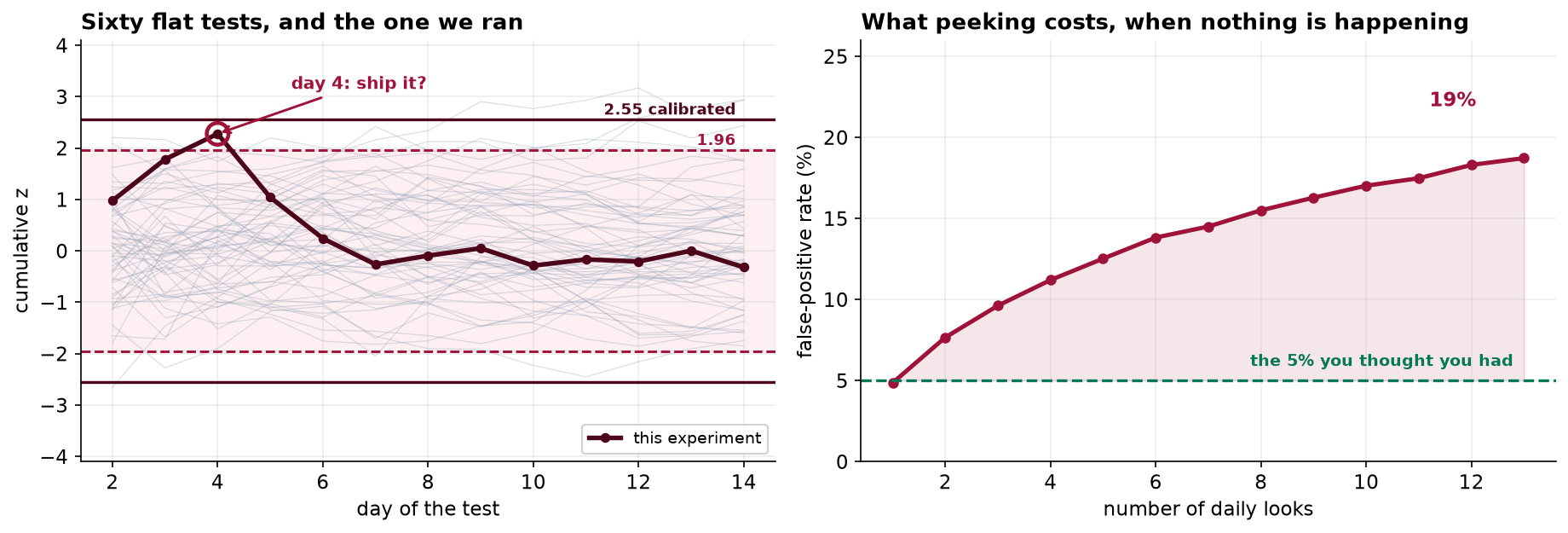
The true lift is zero. On day 4 the treatment led by 15.3 percent at p = 0.023, and a team watching a dashboard would have shipped. At the pre-registered end the lift is −1.1 percent at p = 0.75. Simulation puts the chance of at least one significant day, on a test where nothing is happening, at 18.7 percent.
The Plan, Written Before the Traffic
Twelve decisions, all made on day 0 and all recorded on the ExperimentPlan sheet of the workbook.
They are the reason this test can be defended afterward, and several of them become impossible to make honestly
the moment a result is visible.
| Line | Decision | Why it has to be fixed in advance |
|---|---|---|
| P2 Primary metric | Conversion rate, orders per assigned visitor. One metric. | Choosing the metric after seeing which one moved is the oldest trick there is |
| P4 MDE | A 10 percent relative lift, 4.00 percent to 4.40 percent | Sets the sample size, and encodes what the business would actually act on |
| P5 Power | 80 percent at α = 0.05, two-sided | Two-sided because a drop must be detectable too |
| P7 Stopping rule | One analysis, at the planned end | The single most important line on the sheet |
| P10 Exclusions | Duplicate rows, cross-arm visitors, refund sentinels | Named before anyone knows which direction dropping them moves the result |
| P11 Secondaries | Reported as intervals, never as tests | Stops a null primary being rescued by a hunt through the rest |
Read P4 and P7 together, because between them they turn this from a search into an experiment. P4 says that a lift below 10 percent is not worth having, which is a judgment about build cost and margin that no statistician can supply. P7 says there will be exactly one analysis. Neither line is difficult to write. Both are nearly impossible to write after the fact.
How Big, and How Long
Four numbers determine the sample size, and none of them comes from the data: the baseline rate, the smallest effect worth detecting, the power, and the significance level. At a 4.0 percent baseline and a 10 percent relative MDE, with 80 percent power at α = 0.05, the requirement is 39,472 visitors per arm, or 78,944 in total. At roughly 5,700 visitors a day that is 13.8 days, so the plan says 14.
The interesting part is what happens if the business asks for more sensitivity. Because n scales with the inverse square of the effect, the cost of caring about smaller lifts rises brutally.
| Relative MDE | Detects | n per arm | Days at 5,700 per day |
|---|---|---|---|
| 20% | 4.00% to 4.80% | 10,313 | 4 |
| 15% | 4.00% to 4.60% | 17,940 | 6 |
| 10% (used) | 4.00% to 4.40% | 39,472 | 14 |
| 7% | 4.00% to 4.28% | 79,458 | 28 |
| 5% | 4.00% to 4.20% | 154,301 | 54 |
| 3% | 4.00% to 4.12% | 424,617 | 149 |
Chasing a 3 percent lift would take 149 days. By then the site, the season and the audience have all changed, so the thing being measured is no longer the thing that was launched. A test that cannot finish inside a stable period is not a cheaper test, it is an unanswerable one, and saying so is more useful to the business than quietly running it anyway.
A test with 30 percent power does not merely fail to find real effects. When it does reach significance, the estimate it reports is inflated, because only the largest random excursions clear the bar. That is the winner's curse, and it is why a string of underpowered wins produces a roadmap of changes that never replicate.
The Log, and What Comes Out of It
A real assignment log is not a tidy table. Four faults here, and all four were named in P10 of the plan before anyone knew which direction removing them would push the answer.
| Step | Rows | What happened |
|---|---|---|
| Raw log | 80,236 | One row per assignment event, not per visitor |
| Drop duplicate rows | 79,896 | 340 removed: the logger retried on timeout |
| Drop cross-arm visitors | 79,704 | 192 rows from 96 visitors who saw both checkouts |
| One row per visitor | 79,704 | The analysis file |
| Void refund sentinels | 120 values | A revenue of −1 means refunded, not a negative sale |
The cross-arm visitors are the exclusion worth dwelling on. Ninety-six people were bucketed into both arms by a bug. The tempting repair is to keep whichever assignment came first, which sounds harmless and quietly converts a randomized comparison into a comparison of whoever happened to get logged twice. They belong to neither arm, so they leave both. Ninety-six out of eighty thousand costs nothing; the principle costs nothing either, and it is the same principle that would matter if the bug had touched nine thousand.
The Health Check That Comes First
Before a single outcome is examined, check that the randomization did what it claimed. Assignment was 50/50, so the two arms should be the same size to within chance. If they are not, something in the bucketing or the logging is broken, and every number downstream is suspect no matter how good it looks.
That is what a healthy randomization looks like. Note that the threshold for this particular test is deliberately strict rather than loose: practitioners typically act only below p = 0.001 or so, because the sample is enormous and you want the alarm to fire on genuine pipeline faults rather than on ordinary noise. Note also the order. Running the SRM check after seeing the conversion numbers invites the analyst to decide how seriously to take it based on whether they liked the result.
Both arms clear the 39,472 the plan required, so the test has the power it was designed with. That is worth stating explicitly, because a test that ends short of its planned n is a different test from the one that was specified, and its result should be reported as such.
The Day-4 Result That Would Have Shipped
The team has a dashboard. On day 4 it shows a win, and not a marginal one.
| Day 4, the peek | Day 14, the planned end | |
|---|---|---|
| Visitors | 22,773 | 79,704 |
| Control | 4.0056% | 4.1102% |
| Treatment | 4.6185% | 4.0652% |
| Relative lift | +15.30% | −1.09% |
| 95% interval | [+2.13%, +28.47%] | [−7.78%, +5.59%] |
| Test | z = 2.277, p = 0.0228 | z = −0.321, p = 0.7484 |
Significant, and comfortably above the 10 percent bar that justified building the thing. Every instinct says ship it and move on to the next project. The only thing standing in the way is a line in a document saying the test runs for 14 days, written by people who had not yet seen this number.
Look at what happens to the effect over the following ten days. It does not shrink toward zero, which is what most people expect. It changes sign. Two thirds of the eventual traffic arrived after the moment the team would have stopped, and it carried the estimate back to where the truth is, which is nowhere.
How Often Day 4 Happens by Accident
One run proves nothing, and it would be dishonest to build a chapter on a single lucky draw. The question that can be answered properly is this: if the treatment does nothing at all, how often does a team that checks daily see at least one significant result? That is a simulation, not an argument.
Five thousand experiments were generated with a true lift of exactly zero, each accumulating 2,850 visitors per arm per day for 14 days, and each tested at the end of every day from day 2 onward.
| How the test was run | Declared significant |
|---|---|
| One analysis, at the planned end | 4.7% |
| Checking after 3 days | 9.6% |
| Checking after 6 days | 13.8% |
| Checking after 9 days | 16.3% |
| Checking every day, 13 looks | 18.7% |
Five percent becomes nearly nineteen. The significance level you chose applies to one comparison, and thirteen looks at the same accumulating data is thirteen chances to cross the line. The looks are heavily correlated, since each one contains all the data from the last, which is why the rate lands near 19 percent rather than the 49 percent you would get from thirteen unrelated tests. Almost one flat test in five can be declared a winner by a team doing nothing more sinister than watching a dashboard.
Nobody in this story did anything dishonest. There was no fishing through metrics, no dropping of awkward segments, no reruns with different filters. A team looked at its own dashboard and stopped when the answer looked clear. That is the point: the failure is structural, so the remedy has to be structural too.
A Stopping Rule That Survives Being Watched
Monitoring is not the sin. Monitoring against a boundary built for a single look is. Teams have perfectly good reasons to watch a running experiment, not least catching a change that is actively harming customers. The fix is to decide in advance that you will look, and to widen the boundary so that the error rate across the whole sequence is the one you wanted.
The same simulation that exposed the problem sets the threshold. Take the largest absolute z each simulated experiment ever reaches across its 13 looks, and find the 95th percentile of that distribution.
The day-4 z of 2.28 clears 1.96 and does not clear 2.55. A team that had written this boundary into its plan would have looked at the dashboard on day 4, seen a 15 percent lift, noted that it had not crossed the line, and kept the test running. That is precisely the behavior the wider boundary is being paid for.
Note how much less severe the calibrated boundary is than a naive correction. Treating the 13 looks as independent, a Sidak adjustment would demand p < 0.0039 at each one. The looks are nested, not independent, so simulating the actual correlation buys back most of that severity: 0.011 rather than 0.0039. Published group-sequential designs such as Pocock and O'Brien-Fleming boundaries are the formal versions of the same idea, and O'Brien-Fleming in particular spends its error unevenly, staying very strict early and relaxing toward the planned end.
CUPED: The Same Precision on Less Traffic
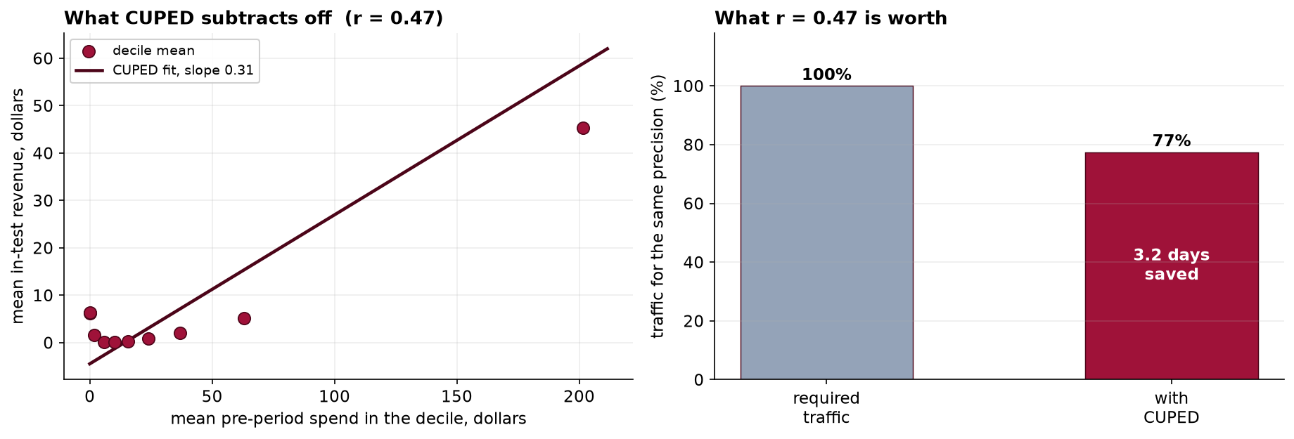
Sample size is set by variance, so anything that removes variance without touching the treatment effect buys traffic back. CUPED, controlled experiment using pre-experiment data, subtracts off the part of the outcome that was predictable from behavior recorded before assignment. Because the covariate predates the treatment, nothing the treatment did can have influenced it, which is what makes the subtraction safe.
Here the outcome is revenue per visitor and the covariate is spend in the 30 days before assignment. They correlate at r = 0.475.
CUPED buys you exactly r squared, and not one point more. That single fact is worth carrying around, because it tells you before you build anything whether the technique is worth the pipeline. A covariate correlated 0.475 with the outcome removes 22.5 percent of the variance. A covariate correlated 0.15 removes 2 percent and is not worth a meeting. In this book's own data the same method applied to the conversion metric rather than revenue would have been close to worthless, because a rare binary outcome is barely predictable from anything.
Notice what CUPED does not do. It does not change the estimate, only its precision. The adjusted and unadjusted differences agree; the adjusted one is measured more sharply. A variance-reduction method that moved the point estimate would be a red flag, not a feature.
The Result, Reported as an Estimate
A p-value of 0.75 is not the finding. The finding is the interval, because the interval is what answers the question the business actually asked, which was never "is the effect exactly zero" but "is it big enough to be worth having".
This is a well-powered null, and it is worth as much as a win. The test was designed to detect a 10 percent lift. The data are consistent with anything from a 7.8 percent drop to a 5.6 percent rise, and the entire interval sits below the bar the business set. The honest conclusion is not "we failed to find an effect", which sounds like a failure of the analysis. It is "we have ruled out an effect large enough to be worth having", which is a genuine answer to the question that was asked.
That conclusion is available only because the sample size was fixed in advance against a stated MDE. Had the test been run to an arbitrary two weeks with no power calculation, the same interval would have been uninterpretable: nobody could have said whether it was narrow enough to rule anything out. The pre-registration is what converts a null result from an absence of news into information.
Revenue per visitor came in at $6.51 in control and $7.09 in treatment. It is tempting to reach for that as a consolation prize. P11 forbids it, for the reason Capstone 4 established: a null primary followed by a search through secondaries is the multiple-comparisons problem wearing different clothes. The right treatment is to report the number with its interval, note that it was not the metric the test was powered for, and let it inform the next experiment's hypothesis rather than this one's conclusion.
What to Watch
- ✓A stopping rule chosen after seeing data is not a stopping rule. "We will run it until it is significant" is not a plan, it is a guarantee of a false positive given enough patience.
- ✓Report the sequence, not just the moment you stopped. The same p = 0.023 means one thing at a planned analysis and something much weaker as the best of thirteen looks. A p-value without its stopping rule cannot be interpreted.
- ✓Publish nulls internally. Teams that only write up wins build a library in which every idea worked, which is how an organization comes to believe things that are not true.
- ✓Watch for novelty and primacy effects. A change can move behavior for a week simply by being new. A 14-day window is partly a defense against reporting that as a permanent lift.
- ✓Check the unit of randomization matches the unit of analysis. Randomizing by visitor and analyzing by session inflates n and shrinks every standard error, which is the design effect of Capstone 18 arriving through a different door.
- ✓Experiments are run on people. Nobody asked these visitors whether they wanted a redesigned checkout, which is normally uncontroversial and stops being so the moment the manipulation touches price, credit or safety. The threshold question is whether you would be comfortable describing the test to the people in it.
Experiment Design in Data Science & AI
Online controlled experiments are the largest applied statistics operation in the world, and every large platform has rediscovered the contents of this chapter the expensive way.
| Where it appears | The same problem, in a different costume |
|---|---|
| Recommender ranking tests | Metrics are heavily skewed by a few users, so variance reduction is the difference between a feasible test and an impossible one |
| Model rollouts | A new model is shipped behind a flag and monitored continuously, which is peeking unless a boundary was set |
| Bandits and adaptive allocation | Traffic is reallocated toward the winner as evidence accrues, which is deliberate peeking with the inference rebuilt to match |
| Interleaving experiments | Both rankings shown to the same user, which removes between-user variance the way pairing did in Capstone 3 |
| LLM evaluation | Pairwise preference judgments on a shared prompt set, with the same MDE and power questions and usually none of the answers |
CUPED comes from Deng, Xu, Kohavi and Walker at Microsoft in 2013, and the variance reduction it reports on real telemetry is broadly what this chapter reproduces. The sequential problem has two modern answers worth knowing: always-valid inference based on confidence sequences, which lets you look continuously with no boundary calculation at all, and group-sequential designs borrowed from clinical trials, where the same logic has been standard since the 1970s. The clinical-trials literature is where an experimenter should look first, because medicine had strong reasons to solve stopping rules honestly long before anybody was testing checkout buttons.
The full project, step by step
The companion notebook reads the pre-registered plan before touching the data, derives the sample size from first principles and tabulates what a smaller MDE would have cost, cleans four faults out of the assignment log, runs the sample ratio mismatch check, reproduces the day-4 result and the day-14 one, simulates five thousand flat experiments to price peeking at 18.7 percent, calibrates the sequential boundary from that same simulation, and implements CUPED from scratch.
The dataset
(capstone-designing-an-ab-test.xlsx) holds the 80,236-row assignment log with its duplicates,
cross-arm visitors and refund sentinels intact, the pre-registration written on day 0, and the true effect that
was simulated so you can check your work. Two written reports accompany it: a plain-language
brief for the product lead who wants to ship, and a technical report covering the
power calculation, the sequential boundary and the variance reduction.
🎓 Key Takeaways
- ✓The MDE sets everything, and it is a business decision. n scales with its inverse square: 10 percent needs 14 days, 3 percent needs 149.
- ✓Peeking turns 5 percent into 18.7 percent. Thirteen daily looks at a test with no effect declared a winner almost one time in five.
- ✓Look all you like, against the right boundary. Calibrating by simulation gave 2.55 rather than 1.96, and the day-4 result of 2.28 would not have stopped the test.
- ✓CUPED buys exactly r squared. A covariate correlated 0.475 with the outcome removed 22.5 percent of the variance and 3.2 days of traffic.
- ✓A well-powered null is a real answer. The interval of −7.8 to +5.6 percent excludes the 10 percent lift that justified the build, which settles the decision.