Association Between Residential Area Type and Commute Mode
A chi-square test of independence on a stratified survey sample.
Keywords: chi-square test of independence; contingency table; expected counts; Cramer's V; standardized residuals; stratified sampling.
1. Introduction
Where both variables of interest are categorical, the data reduce to a contingency table of counts and the question of interest becomes association rather than difference in means. The Pearson chi-square test of independence evaluates whether the joint distribution factorizes into its marginals, that is, whether the conditional distribution of one variable is the same at every level of the other.
The hypotheses are H₀: commute mode and area type are independent, against H₁: they are associated, evaluated at α = 0.05. Because a rejection is uninformative about structure, the analysis is specified in advance to include an effect-size measure and a residual decomposition.
2. Data and sampling design
The instrument comprised five items spanning four measurement types: two nominal (area type, main commute mode), one continuous (age), one ordinal seven-point Likert (commute satisfaction), and one open text. Only the two nominal items enter this analysis.
The sample was stratified by area type with equal allocation, 200 respondents drawn at random within each of four strata. Equal allocation maximizes precision for between-stratum comparison but renders the pooled sample non-representative of the population distribution, a constraint carried through to the Discussion.
| Step | Rule | Removed | Remaining |
|---|---|---|---|
| Raw export | — | — | 802 |
| Normalize labels | trim and case-fold region | 0 | 802 |
| De-duplication | drop duplicate rows | 2 | 800 |
| Complete on both items | drop rows missing region or mode | 5 | 795 |
3. Methods
Observed counts were cross-tabulated and expected counts computed under independence as the outer product of the marginal proportions scaled by n. The expected-count condition (all cells ≥ 5) was verified before testing; had it failed, Fisher's exact test or category collapsing would have been substituted. The Pearson chi-square statistic was computed with (r − 1)(c − 1) degrees of freedom. Association strength was summarized by Cramer's V = sqrt(χ² / (n · min(r−1, c−1))). Standardized Pearson residuals, (O − E)/sqrt(E), were examined cell-by-cell as an omnibus-test decomposition. Analyses used SciPy in Python 3.
4. Results
| Area type | Car | Public transit | Bicycle | Walk | Row total |
|---|---|---|---|---|---|
| Urban Core | 57 (28.5%) | 78 (39.0%) | 33 (16.5%) | 32 (16.0%) | 200 |
| Inner Suburb | 113 (57.1%) | 50 (25.3%) | 14 (7.1%) | 21 (10.6%) | 198 |
| Outer Suburb | 155 (78.3%) | 27 (13.6%) | 9 (4.5%) | 7 (3.5%) | 198 |
| Rural | 178 (89.4%) | 6 (3.0%) | 8 (4.0%) | 7 (3.5%) | 199 |
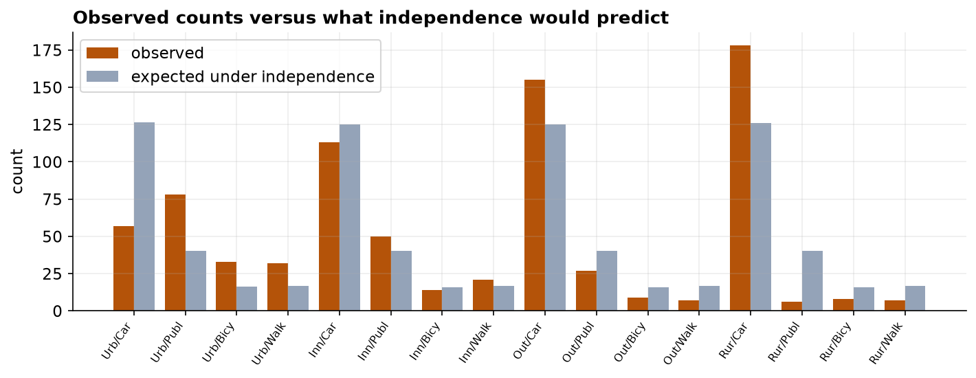
Expected counts under independence ranged from 15.94 to 126.54, satisfying the approximation condition with substantial margin. Note the condition applies to expected rather than observed counts: the Rural × Public transit cell contains only 6 observations yet has an expected count of 40.3.
| Quantity | Value |
|---|---|
| Pearson χ² | 189.70 |
| Degrees of freedom | 9 |
| p-value | 4.75e-36 |
| n | 795 |
| Cramer's V | 0.282 (moderate) |
| Minimum expected count | 15.94 |
The null hypothesis of independence is rejected decisively. Given n = 795, however, statistical significance is a weak criterion; the effect size is the informative quantity, and Cramer's V = 0.282 places the association in the moderate range, substantial for behavioral survey data. The residual decomposition (Table 4) shows that the association is structured rather than diffuse.
| Cell | Observed | Expected | Standardized residual |
|---|---|---|---|
| Urban Core × Car | 57 | 126.5 | -6.18 |
| Urban Core × Public transit | 78 | 40.5 | +5.89 |
| Rural × Car | 178 | 125.9 | +4.64 |
| Rural × Public transit | 6 | 40.3 | -5.40 |
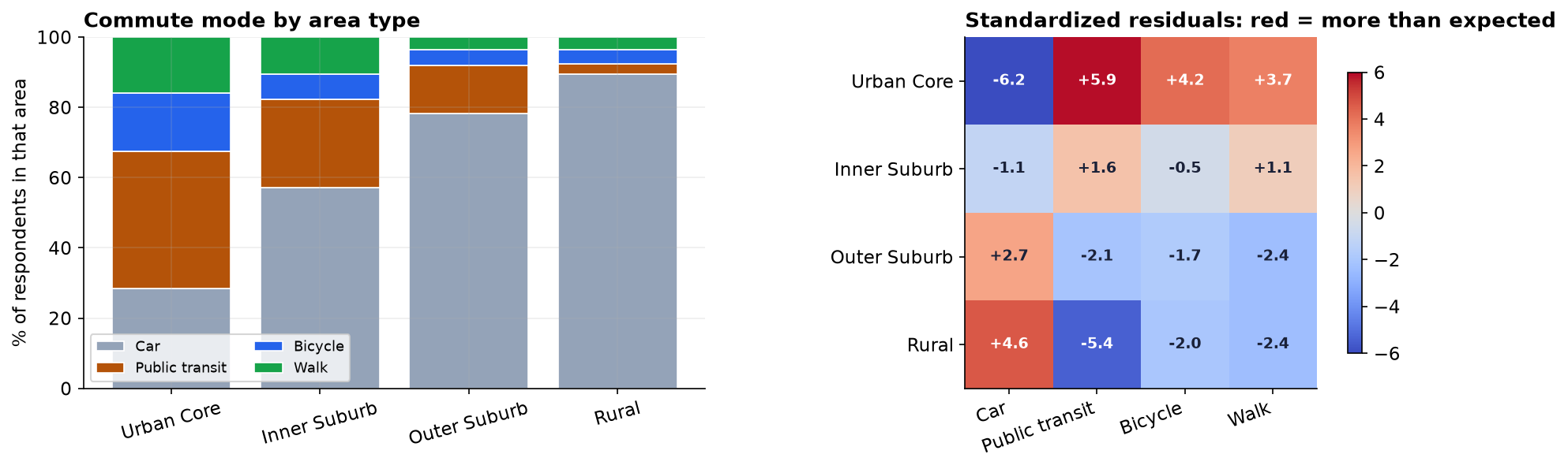
Bicycle and walking cells carry residuals of small magnitude throughout, so the association is attributable almost entirely to substitution between private car and public transit along the density gradient.
5. Interval estimates and confounding assessment
| Quantity | Estimate | 95% CI | Method |
|---|---|---|---|
| Cramer's V | 0.282 | 0.253 to 0.320 | percentile bootstrap |
| Transit share, Urban Core | 39.0% | 32.5% to 45.9% | Wilson |
| Transit share, Inner Suburb | 25.3% | 19.7% to 31.7% | Wilson |
| Transit share, Outer Suburb | 13.6% | 9.5% to 19.1% | Wilson |
| Transit share, Rural | 3.0% | 1.4% to 6.4% | Wilson |
The association measure is bounded between 0.25 and 0.32, supporting a characterization of moderate strength and excluding a strong one. The stratum-specific proportions are the quantities likely to be transferred into planning documents, and each carries a margin of error of six to seven percentage points. Because allocation was equal rather than proportional, these estimates describe the sampled strata and are not population estimates without weighting.
Two covariates recorded in the instrument were not analyzed in the original report. Respondent age differs neither across regions (p = 0.58) nor across modes (p = 0.88), and therefore satisfies neither condition required of a confounder. Commute satisfaction does not differ detectably across modes (H = 1.22, p = 0.75), although the observed ordering places cyclists highest.
The latter result is instructive precisely because it is null. Had it reached significance, a causal reading would still not follow: proximity to the workplace determines both the feasibility of cycling and the pleasantness of the commute, and distance was not measured. A significant test of independence establishes covariation between two categorical variables and is silent on which is antecedent, or whether a third is antecedent to both.
6. Discussion
Commute mode is systematically associated with residential area type, in a monotone gradient consistent with transit availability and trip distance. The practical implication is that a spatially uniform transport intervention is poorly matched to any of the four strata.
Three limitations bound the inference. First, and most consequential for reporting, the equal-allocation design means the pooled sample does not estimate population marginals; any region-wide share must be computed with stratum weights proportional to population, and an unweighted marginal would be biased toward the smaller strata. Between-stratum comparison, which is the object of this analysis, is unaffected. Second, the design is observational and cross-sectional, so the association cannot distinguish preference from availability; a rural respondent reporting car use may face no alternative, and the analysis cannot separate constrained from unconstrained choice. Third, both variables were self-reported on a voluntary instrument, and the forced single-mode response misclassifies multi-modal commuters.
The categorical scheme itself is a modeling decision made before analysis. The four area labels are administrative and the four modes exhaustive only by construction; a finer partition could reveal structure that the present collapsing conceals.
7. Conclusion
Area type and commute mode are not independent, χ²(9) = 189.70, p < 0.001, Cramer's V = 0.282. The association is a monotone density gradient localized to the car and public-transit categories. Findings support stratum-specific transport planning; they do not support pooled regional estimates without population weighting.
References
- Pearson, K. (1900). On the criterion that a given system of deviations from the probable... Philosophical Magazine, 50(302), 157–175.
- Cramer, H. (1946). Mathematical Methods of Statistics. Princeton University Press.
- Agresti, A. (2013). Categorical Data Analysis (3rd ed.). Wiley.
- Haberman, S. J. (1973). The analysis of residuals in cross-classified tables. Biometrics, 29(1), 205–220.
- Cochran, W. G. (1977). Sampling Techniques (3rd ed.). Wiley.
- Fisher, R. A. (1922). On the interpretation of chi-square from contingency tables. JRSS, 85(1), 87–94.
Reproducibility
The dataset (capstone-commute-mode-by-region.xlsx), including the questionnaire and sampling sheets, and an executable notebook reproducing every statistic, table, and figure accompany the chapter. Analyses use NumPy, pandas, SciPy, and Matplotlib.