Change in Cognitive Performance Across a Twelve-Week Training Program
A one-way repeated-measures analysis of variance with Greenhouse-Geisser correction.
Keywords: repeated-measures ANOVA; sphericity; Mauchly's test; Greenhouse-Geisser; attrition bias; within-subject design.
1. Introduction
Within-subject designs increase precision by removing stable between-person variation, but they impose structure on the error covariance. With two conditions this is immaterial, since only one difference exists. With k ≥ 3 conditions the repeated-measures ANOVA additionally assumes sphericity: equality of the variances of all pairwise differences among conditions. Violations inflate the type-I error rate of the uncorrected F test, and are common whenever variability grows over time.
The hypotheses are H₀: μ₁ = μ₂ = μ₃ = μ₄ against H₁: at least one timepoint mean differs, evaluated at α = 0.05. A secondary and more informative objective is to characterize where in the twelve weeks any change occurs.
2. Data
Records comprise a participant identifier, a timepoint, and a composite cognitive score bounded 0 to 100. After removing duplicate rows, missing scores, and out-of-range values, participants lacking any of the four assessments were excluded, as required by a complete-case repeated-measures analysis (Table 1).
| Step | Rule | Result |
|---|---|---|
| Raw export | — | 165 rows |
| De-duplication | drop duplicate rows | 163 rows |
| Missing scores | drop blank cognitive_score | 160 rows |
| Range filter | retain 0 < score ≤ 100 | 158 rows |
| Complete cases | retain participants with all 4 timepoints | 35 of 42 participants (7 excluded) |
3. Methods
Sphericity was evaluated by Mauchly's test, supported by direct inspection of the six pairwise difference variances. Because sphericity was rejected, the Greenhouse-Geisser correction was applied, multiplying both numerator and denominator degrees of freedom by the estimated ε. Effect size is reported as generalized eta-squared, which is preferred to partial eta-squared in repeated-measures designs because it is comparable across designs. Pairwise contrasts across all six timepoint pairs used paired tests with Holm correction, and Hedges' g quantified each contrast. The Friedman test served as a distribution-free sensitivity analysis. Analyses used pingouin and SciPy in Python 3.
4. Results
| Timepoint | n | Mean | SD | Change from baseline |
|---|---|---|---|---|
| Baseline | 35 | 51.84 | 8.73 | — |
| Week 4 | 35 | 56.38 | 10.00 | +4.54 |
| Week 8 | 35 | 56.99 | 11.49 | +5.14 |
| Week 12 | 35 | 57.87 | 13.90 | +6.02 |
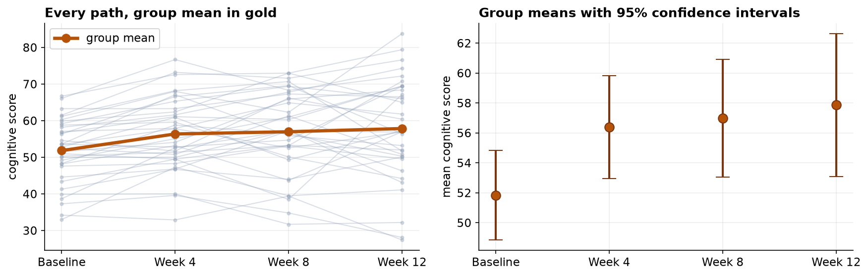
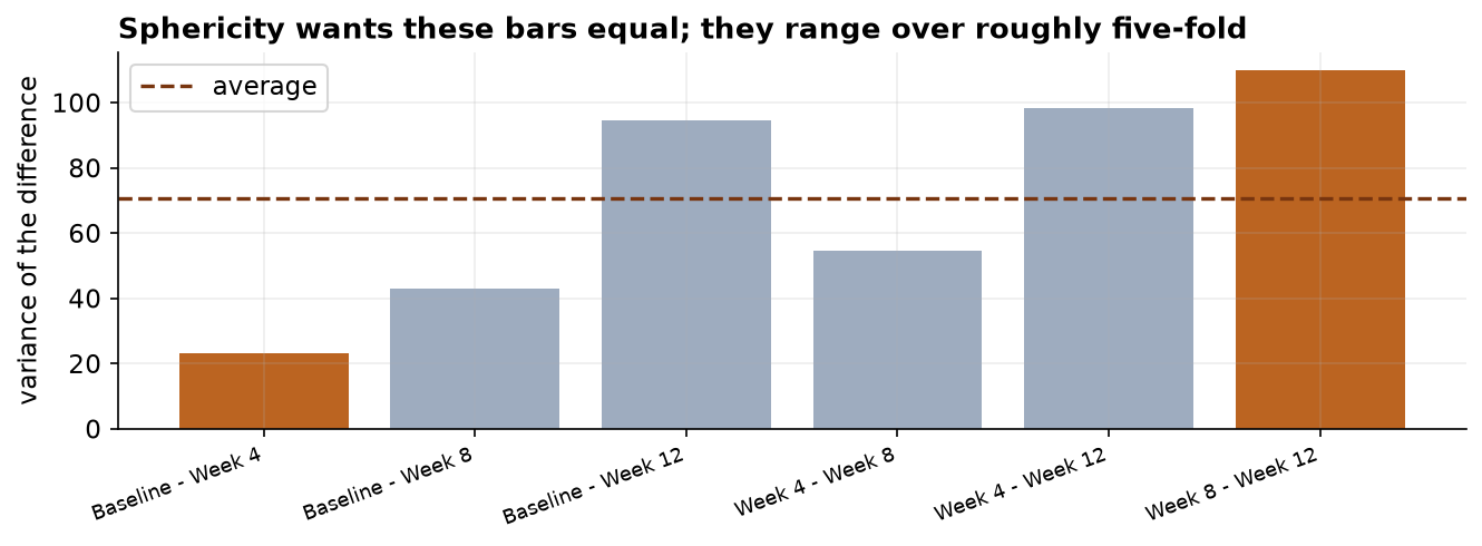
Dispersion increased monotonically across timepoints (SD 8.73 to 13.90), which anticipates the sphericity failure. The six pairwise difference variances span 23.1 to 109.9, a ratio of 4.8, and Mauchly's test rejects sphericity (W = 0.477, p = 0.0002).
| Pair | Variance of the difference |
|---|---|
| Baseline vs Week 4 | 23.1 |
| Baseline vs Week 8 | 42.9 |
| Baseline vs Week 12 | 94.6 |
| Week 4 vs Week 8 | 54.7 |
| Week 4 vs Week 12 | 98.3 |
| Week 8 vs Week 12 | 109.9 |
| Quantity | Uncorrected | Greenhouse-Geisser corrected |
|---|---|---|
| Degrees of freedom | (3, 102) | (2.12, 72.00) |
| F | 7.163 | 7.163 |
| p | 2.06e-04 | 0.0012 |
| ε | — | 0.706 |
| Generalized η² | 0.0426 | 0.0426 |
The omnibus null is rejected under the corrected test, F(2.12, 72.00) = 7.16, p = 0.0012. The correction raised the p-value by roughly an order of magnitude without altering the conclusion, which is the desired outcome but not one that can be assumed in advance. The Friedman test agreed (χ² = 22.74, p = 4.57e-05). Generalized η² = 0.043 indicates a modest proportion of total variance attributable to timepoint.
| Contrast | Hedges' g | Uncorrected p | Holm-adjusted p | Decision |
|---|---|---|---|---|
| Baseline vs Week 12 | -0.513 | 0.0008 | 0.0034 | reject H₀ |
| Baseline vs Week 4 | -0.478 | 0.0000 | 0.0000 | reject H₀ |
| Baseline vs Week 8 | -0.498 | 0.0000 | 0.0002 | reject H₀ |
| Week 12 vs Week 4 | +0.121 | 0.3825 | 1.0000 | retain H₀ |
| Week 12 vs Week 8 | +0.068 | 0.6227 | 1.0000 | retain H₀ |
| Week 4 vs Week 8 | -0.055 | 0.6327 | 1.0000 | retain H₀ |
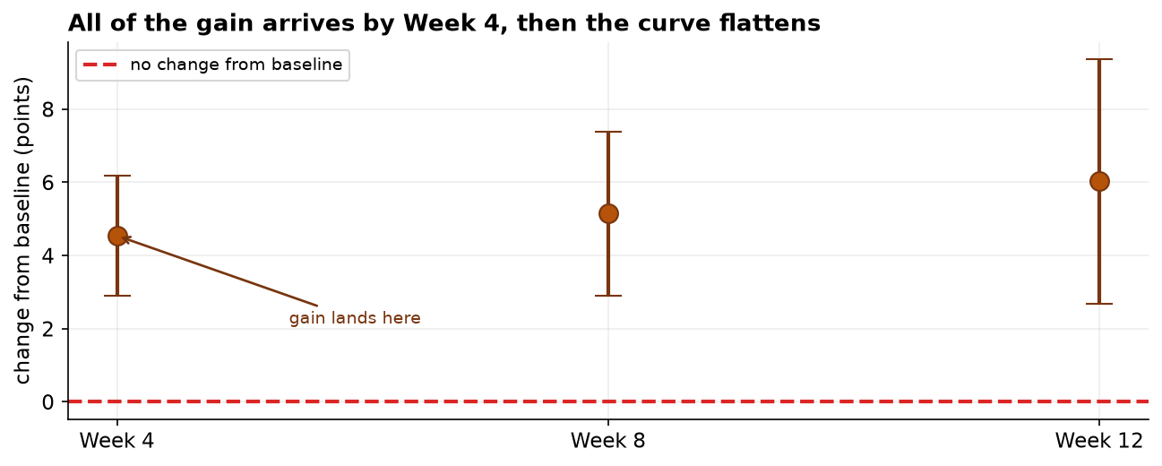
The contrast structure is the substantive result. Every comparison against Baseline is significant after correction, while no comparison among the three follow-up timepoints is even nominally significant. The temporal profile is therefore a step rather than a trend: the effect is realized within the first four weeks and does not accumulate thereafter.
5. Interval estimates
| Contrast | Mean change | 95% CI |
|---|---|---|
| Baseline to week 4 | +4.54 | +2.89 to +6.19 |
| Baseline to week 8 | +5.14 | +2.89 to +7.39 |
| Baseline to week 12 | +6.02 | +2.68 to +9.36 |
| Week 4 to week 12 | +1.48 | −1.92 to +4.89 |
Each interval measured from baseline excludes zero, establishing improvement at every assessment point. The final row is the contrast of program-design interest and was not reported in the original analysis: the increment accruing between week 4 and week 12 has an interval containing zero.
The post-hoc comparisons already indicated that the three post-baseline timepoints were mutually indistinguishable. Expressing the same result as an interval converts a non-rejection into a bounded estimate: the additional eight weeks of intervention produced a change of at most approximately 4.9 points and possibly a decrement. For a sponsor selecting between a four-week and a twelve-week protocol this is the operative finding, and it is not visible in the omnibus test.
6. Discussion
Cognitive performance improved across the program, and the inference survives correction for a materially violated sphericity assumption. The practically important result is the profile rather than the omnibus test: approximately 4.5 points are gained in the first four weeks, with no detectable accrual over the remaining eight. If measurable cognitive gain is the program objective, this is evidence for a shorter, more intensive design.
Threats to validity are substantial and structural. First, attrition: 7 participants were excluded for incomplete records, and complete-case analysis is unbiased only under a missing-completely-at-random mechanism. If non-responders discontinued because they were not improving, the retained sample is enriched for responders and the estimate is optimistic. Comparison of excluded and retained participants on baseline and early-change measures is the minimum diagnostic; a linear mixed-effects model, which accommodates partial records and does not require sphericity, is the preferred analysis under informative dropout.
Second, the design is single-arm. Repeated administration of a similar instrument produces practice effects that are observationally indistinguishable from genuine cognitive gain, and regression to the mean will operate if participants were recruited on low baseline performance. Neither is estimable without a concurrent control group. Third, the retained nulls among the follow-up contrasts should not be interpreted as establishing no further change; with N = 35 the design has limited power for small increments, and a ceiling on the instrument would produce the same pattern.
7. Conclusion
Cognitive scores changed significantly across four timepoints, F(2.12, 72.00) = 7.16, p = 0.0012 after Greenhouse-Geisser correction, generalized η² = 0.043. Post-hoc contrasts localize the entire effect to the Baseline-to-Week-4 interval. Given the single-arm design and the exclusion of 7 participants for incomplete data, the estimate should be regarded as an upper bound pending a controlled study analyzed with a method robust to informative dropout.
References
- Mauchly, J. W. (1940). Significance test for sphericity of a normal n-variate distribution. Annals of Mathematical Statistics, 11(2), 204–209.
- Greenhouse, S. W., & Geisser, S. (1959). On methods in the analysis of profile data. Psychometrika, 24(2), 95–112.
- Huynh, H., & Feldt, L. S. (1976). Estimation of the Box correction for degrees of freedom. Journal of Educational Statistics, 1(1), 69–82.
- Olejnik, S., & Algina, J. (2003). Generalized eta and omega squared statistics. Psychological Methods, 8(4), 434–447.
- Holm, S. (1979). A simple sequentially rejective multiple test procedure. Scandinavian Journal of Statistics, 6(2), 65–70.
- Friedman, M. (1937). The use of ranks to avoid the assumption of normality. JASA, 32(200), 675–701.
- Little, R. J. A., & Rubin, D. B. (2019). Statistical Analysis with Missing Data (3rd ed.). Wiley.
Reproducibility
The dataset (capstone-cognitive-training-over-time.xlsx) and an executable notebook reproducing every statistic, table, and figure accompany the chapter. Analyses use NumPy, pandas, SciPy, pingouin, and Matplotlib.