Comparing Three Instructional Formats on Final Examination Performance

A one-way analysis of variance with Tukey HSD post-hoc comparisons.

Author John Fisher

Series Statistics, Data Science and AI: A Visual Handbook

Design Three independent groups, one factor, α = 0.05

Where this comes from

Chapter Chapter 164 · One-Way ANOVA: Three Teaching Methods

Part Part XXVII · Capstone Projects: Statistical Testing

Dataset capstone-teaching-methods-exam-scores.xlsx

Notebook View the analysis

Abstract. Objective. To determine whether final examination performance differs across three instructional formats (Lecture, Blended, Flipped) and, if so, to identify which formats differ. Methods. Examination scores were compared across three independent groups of students (n = 130 after cleaning). Group normality was assessed by Shapiro-Wilk and quantile-quantile plots, and homogeneity of variance by Levene's and Bartlett's tests. A one-way analysis of variance was followed by Tukey's honestly significant difference procedure for pairwise comparisons, with the Kruskal-Wallis test as a distribution-free check. Eta-squared quantified effect size. Results. All groups satisfied normality (Shapiro-Wilk p = 0.66, 0.95, 0.86) and homogeneity (Levene p = 0.82; Bartlett p = 0.90). The omnibus test was significant, F(2, 127) = 11.07, p = 3.69e-05, η² = 0.149. Tukey comparisons attributed the effect exclusively to the Flipped format, which exceeded Blended by -7.94 points (95% CI [-12.41, -3.47], p = 0.0001) and Lecture by 7.56 points (p = 0.0004); Lecture and Blended did not differ (p = 0.978). Kruskal-Wallis concurred (p = 8.35e-05). Conclusions. The omnibus result is driven by a single format. Reporting the significant F without the post-hoc structure would materially misrepresent the finding. Because assignment was not randomized, the estimate is associational and vulnerable to self-selection and instructor confounding.

Keywords: one-way ANOVA; Tukey HSD; family-wise error rate; homogeneity of variance; eta-squared; educational assessment.

1. Introduction

Comparing more than two conditions on a continuous outcome is the canonical application of analysis of variance. The motivating alternative, conducting all pairwise t-tests, is inadmissible without correction: for three groups the family-wise error rate under independent testing at α = 0.05 is 1 − (1 − 0.05)³ ≈ 14.3%. ANOVA poses a single omnibus question at the nominal level, and a post-hoc procedure then recovers the pairwise detail under family-wise control.

The hypotheses are H₀: μ₁ = μ₂ = μ₃ against H₁: at least one mean differs, evaluated at α = 0.05. It is worth emphasizing that H₁ is an existential claim; rejecting H₀ licenses no statement about any particular pair, which is the precise gap the post-hoc analysis fills.

2. Data

The dataset comprises 137 student records with an instructional-format label, section, and final examination score. The format label was recorded with inconsistent capitalization and trailing whitespace and was normalized before analysis; duplicates, missing outcomes, and out-of-range scores were then removed (Table 1), leaving n = 130 (45 Lecture, 43 Blended, 42 Flipped).

Table 1. Data-cleaning provenance. Removed out-of-range scores: {-5, 127}.

Step	Rule	Removed	Remaining
Raw export	—	—	137
Normalize label	trim and case-fold `method`	0	137
De-duplication	drop duplicate rows	2	135
Missing outcome	drop blank `exam_score`	3	132
Range filter	retain 0 ≤ score ≤ 100	2	130

3. Methods

Normality within each group was assessed by the Shapiro-Wilk test supported by normal quantile-quantile plots. Homogeneity of variance was tested by Levene's test, which is robust to departures from normality, and by Bartlett's test. Because both assumptions were satisfied, the classical fixed-effects one-way ANOVA was used rather than Welch's heteroscedastic variant. Pairwise comparisons employed Tukey's HSD, which controls the family-wise error rate across all three contrasts. The Kruskal-Wallis test provided a distribution-free sensitivity analysis. Effect size was reported as η² = SS_between / SS_total. Analyses used SciPy and statsmodels in Python 3.

4. Results

Table 2. Descriptive statistics and per-group normality by instructional format.

Format	n	Mean	SD	Shapiro-Wilk p
Lecture	45	73.16	8.85	0.659
Blended	43	73.53	9.06	0.952
Flipped	42	81.10	8.45	0.859

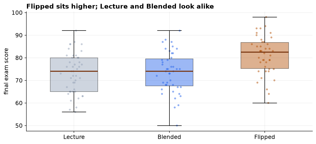
Boxplots of exam score by teaching method with individual student points overlaid; Lecture and Blended sit at the same level while Flipped is higher. — Figure 1. Distribution of examination scores by format, with individual observations overlaid. Lecture and Blended are visually coincident; Flipped is displaced upward.

Homogeneity of variance was supported by both tests (Levene W = 0.200, p = 0.819; Bartlett χ² = 0.204, p = 0.903), with group standard deviations spanning only 8.45 to 9.06. The classical ANOVA is therefore appropriate.

Table 3. One-way analysis of variance for examination score by instructional format. η² = 0.149.

Source	Sum of squares	df	F	p
Between formats	1712.70	2	11.075	3.69e-05
Within (residual)	9820.23	127	—	—

The omnibus null was rejected, F(2, 127) = 11.075, p = 3.69e-05, with η² = 0.149, indicating that instructional format accounts for approximately 15% of variance in examination score. The Kruskal-Wallis test agreed (H = 18.781, p = 8.35e-05), confirming the conclusion does not depend on the normality assumption. Post-hoc comparisons (Table 4) localize the effect.

Table 4. Tukey HSD pairwise comparisons, family-wise error rate controlled at 0.05.

Comparison	Mean difference	95% CI	Adjusted p	Decision
Blended vs Flipped	+7.56	[3.04, 12.08]	0.0004	reject H₀
Blended vs Lecture	-0.38	[-4.83, 4.07]	0.9777	retain H₀
Flipped vs Lecture	-7.94	[-12.41, -3.47]	0.0001	reject H₀

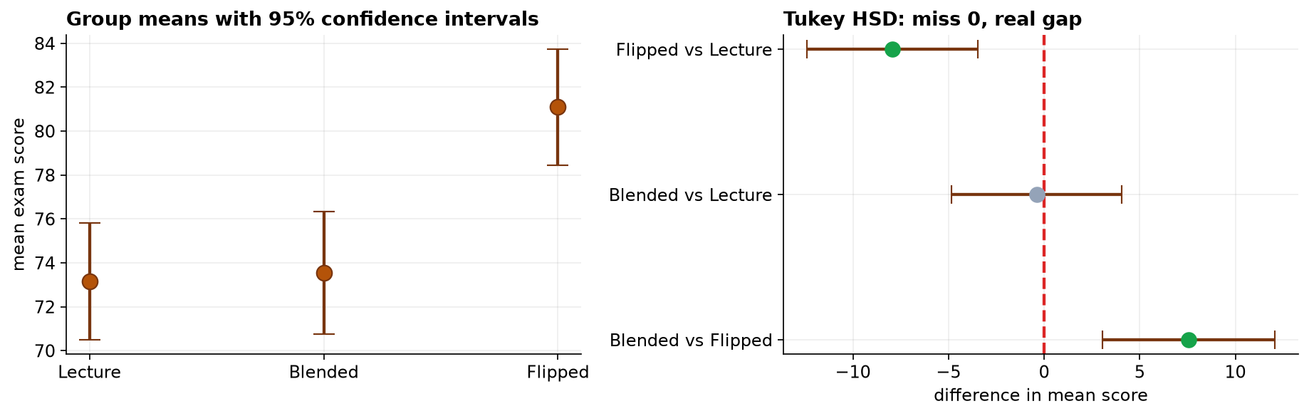
Group means with confidence intervals showing Flipped separated from the other two, and a Tukey difference plot where the two Flipped contrasts exclude zero and the Lecture-Blended contrast includes it. — Figure 2. Left: group means with 95% confidence intervals. Right: Tukey pairwise differences; intervals excluding zero denote significant contrasts.

The post-hoc structure is the substantive result. Both contrasts involving the Flipped format are significant with confidence intervals well clear of zero, whereas the Lecture-Blended contrast is centered near zero with an interval spanning it. The omnibus effect is therefore attributable to a single format rather than to a graded ordering of all three.

5. Interval estimates

Table 5. Tukey-adjusted interval estimates for the pairwise contrasts, and an interval for the effect size.

Contrast	Difference	95% CI	Verdict
Flipped over Lecture	+7.94	+3.47 to +12.41	differs
Flipped over Blended	+7.56	+3.04 to +12.08	differs
Lecture against Blended	−0.38	−4.83 to +4.07	not distinguishable
Eta-squared	0.149	0.063 to 0.279	percentile bootstrap

The Tukey procedure computes these intervals as a matter of course, and reporting only the reject-or-retain decision discards the information they carry. The magnitude of the flipped-classroom advantage is bounded between roughly 3.5 and 12.4 marks, a range across which the institutional case for retraining staff differs substantially.

The non-significant contrast merits particular attention. The interval for Lecture against Blended extends from −4.83 to +4.07, so the data are compatible with an advantage of nearly five marks in either direction. This is an inconclusive result rather than a demonstration of equivalence, and the two are frequently conflated when a p-value is reported without its interval. An equivalence claim would require the interval to fall entirely within a pre-specified region of practical indifference, which it does not.

The interval for eta-squared spans 0.06 to 0.28. The proportion of outcome variance attributable to teaching method is correspondingly imprecise, and the point estimate should not be reported to three decimal places.

6. Discussion

Instructional format is associated with examination performance, but the association is concentrated: the Flipped format exceeds both alternatives by approximately eight points, while Lecture and Blended are statistically indistinguishable. Reporting only the significant omnibus test would imply a three-way ordering that the data do not support, and would misdirect any resulting curricular decision. The magnitude, η² ≈ 0.15, is substantial for an educational intervention while still leaving the majority of variance to student-level factors outside the design.

Threats to validity are primarily structural rather than statistical. Assignment to sections was not randomized, so self-selection is a live alternative explanation: if more prepared or more motivated students preferentially enrolled in Flipped sections, the observed difference would arise with no instructional effect whatsoever. Verification that prior achievement is balanced across formats is a minimal safeguard, and randomization is the definitive one. Instructor effects are similarly entangled with format; unless instructors taught across multiple formats, the two are not separately identifiable. Finally, a single summative examination is a narrow operationalization of learning and says nothing about retention or transfer.

The retained null for the Lecture-Blended contrast should not be read as evidence of equivalence. It indicates only that this design did not detect a difference; formally establishing equivalence would require an equivalence-testing framework with a pre-specified margin.

7. Conclusion

Examination performance differed significantly across three instructional formats, F(2, 127) = 11.07, p < 0.001, η² = 0.149. Tukey HSD attributed the effect wholly to the Flipped format (exceeding Lecture and Blended by approximately 8 points, both adjusted p < 0.001), with no detectable difference between Lecture and Blended (p = 0.98). The finding is robust to a distribution-free check but, given non-randomized assignment, is associational rather than causal.

References

Fisher, R. A. (1925). Statistical Methods for Research Workers. Oliver & Boyd.
Tukey, J. W. (1949). Comparing individual means in the analysis of variance. Biometrics, 5(2), 99–114.
Levene, H. (1960). Robust tests for equality of variances. In Contributions to Probability and Statistics (pp. 278–292). Stanford University Press.
Bartlett, M. S. (1937). Properties of sufficiency and statistical tests. Proc. R. Soc. Lond. A, 160(901), 268–282.
Kruskal, W. H., & Wallis, W. A. (1952). Use of ranks in one-criterion variance analysis. JASA, 47(260), 583–621.
Cohen, J. (1988). Statistical Power Analysis for the Behavioral Sciences (2nd ed.). Lawrence Erlbaum.
Lakens, D. (2017). Equivalence tests. Social Psychological and Personality Science, 8(4), 355–362.

Reproducibility

The dataset (capstone-teaching-methods-exam-scores.xlsx) and an executable notebook reproducing every statistic, table, and figure accompany the chapter. Analyses use NumPy, pandas, SciPy, statsmodels, and Matplotlib.

← Back to Chapter 164 📓 Companion notebook 📊 Download dataset

From Statistics, Data Science and AI: A Visual Handbook by John Fisher. Every statistic, table, and figure in this report is reproduced by the companion notebook.