Unsupervised Detection: Preprocessing Dominates, and the Threshold Is a Constraint
Three detectors shared 4 of 120 alerts. Repairing four data defects and scoping to one operating mode moved precision from under 2 percent to 85. The threshold is set by review capacity, and sensitivity is measured by injection.
1. Data and the evaluation problem
Thirty days of five-minute telemetry from one bottling line, twelve sensors. The export contained 8,736 rows; a clock resync on day 7 had written 96 readings twice, leaving 8,640 after deduplication on day and minute.
There are no historical fault labels, which is the reason the project exists. No ROC curve, no tuned threshold, no accuracy comparison between methods. The dataset used here carries a sealed answer key because it was generated for teaching; all method selection was completed before it was opened, and it is reported in sections 3 to 6 only to establish that the reasoning was sound.
Ground truth, once opened: 934 readings (10.8 percent) fall inside one of 24 fault episodes; 2,388 readings (27.6 percent) are touched by one of the four engineering-log events. The data defects outnumber the faults by more than two to one.
2. Why univariate limits fail
| Rule | Alerts | Per day | Fault readings caught | Precision |
|---|---|---|---|---|
| Any sensor beyond 3 SD | 913 | 30.4 | 67 of 934 (7.2%) | 7.3% |
| Any sensor beyond 4 SD | 11 | 0.4 | 4 of 934 (0.4%) | 36.4% |
The three fault modes are constructed to be individually in-range: bearing wear raises vibration, motor temperature and conveyor current together; valve drift raises fill volume while the control loop lowers valve position; an air leak lowers supply pressure and cap torque while valve position rises to compensate. Each sensor stays within its normal operating band throughout, so the signal exists only in the joint distribution.
3. Three detectors on the raw export
| Detector | Machine faults | Data defects | Neither |
|---|---|---|---|
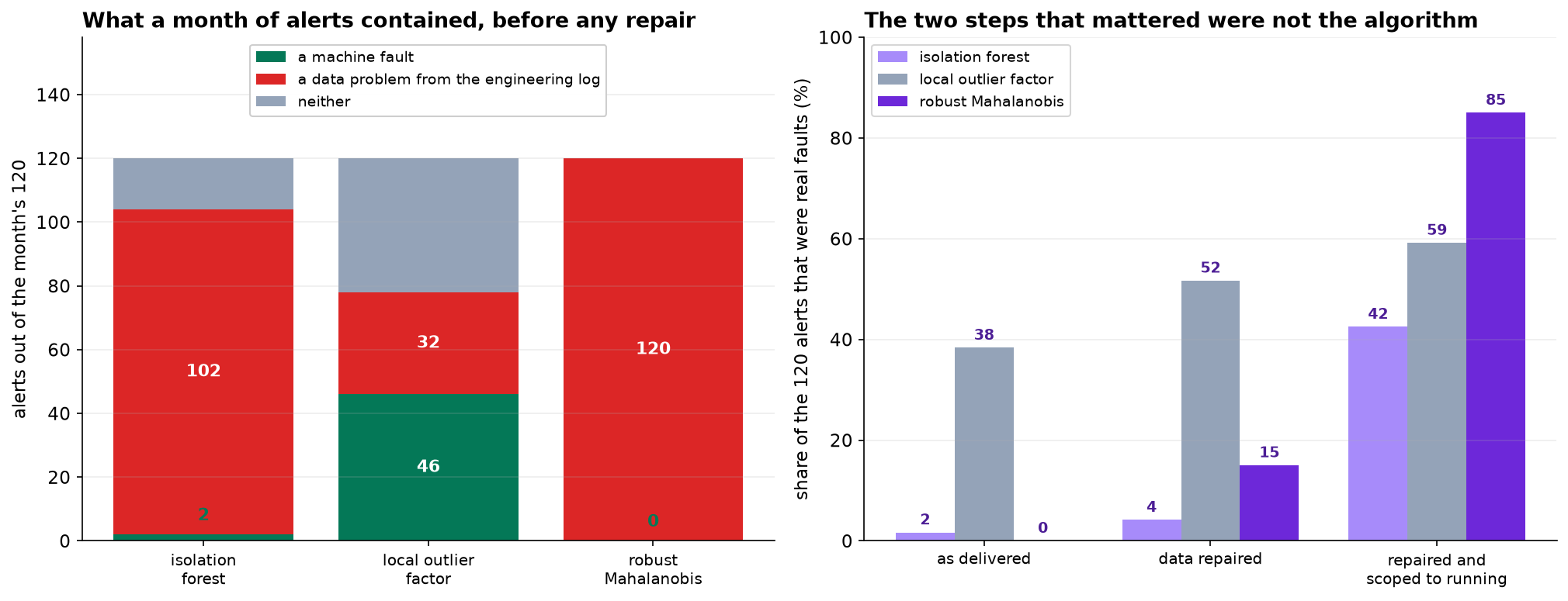
| Isolation forest (400 trees) | 2 | 102 | 16 |
| Local outlier factor (k = 35) | 46 | 32 | 49 |
| Robust Mahalanobis (MCD) | 0 | 120 | 0 |
Ninety of the isolation forest's alerts are the 576 readings where the pressure transmitter reported in psi. Both global methods spend essentially the whole budget on the unit change; LOF does not, because it evaluates density relative to a local neighbourhood and the psi block forms its own dense region of 576 mutually similar points. This is a property of the defect, not a general superiority of LOF, and section 5 shows the ordering reversing once the defect is removed.
4. Inter-method agreement
| Pair | Shared alerts out of 120 | Jaccard |
|---|---|---|
| Isolation forest / LOF | 10 | 0.043 |
| Isolation forest / MCD | 45 | 0.231 |
| LOF / MCD | 4 | 0.017 |
| All three | 4 |
In a supervised setting this disagreement would be resolved by held-out accuracy. Unsupervised, there is no such adjudication, and selecting a method on published benchmark performance is a weak substitute given that benchmark rankings are themselves sensitive to preprocessing. The disagreement is instead exploited directly in section 6.
5. Repairs, scope, and the effect on precision
Four defects, all corresponding to entries in the engineering log:
| Defect | Evidence in the data | Treatment |
|---|---|---|
| Clock resync, day 7 | 96 duplicated (day, minute) keys | Deduplicate |
| Firmware update, day 12 | 576 readings above 20 in a bar-denominated column; median 90.8 vs 6.20, ratio 14.63 | Divide by 14.5038 |
| Sensor not updating, day 19 | 79 readings with zero rolling standard deviation over six samples | Drop |
| Recalibration, day 24 | Median labeler tension 11.75 N before, 14.09 N after | Subtract the 2.34 N step |
After repair, 100 percent of the isolation forest's alerts had line speed below 100 bottles per minute, against 12.1 percent of the file. An idle line is a distinct operating mode: speed near zero, motor temperature relaxing toward ambient, vibration at a background level. It is correctly identified as atypical and is not a fault. Analysis was restricted to the 7,529 readings with the line running, of which 907 (12.0 percent) are during a fault.
| Detector | As delivered | Data repaired | Repaired and scoped |
|---|---|---|---|
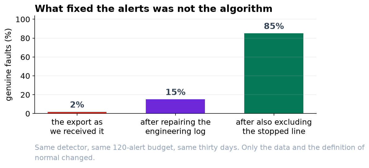
| Isolation forest | 1.7% | 4.2% | 42.5% |
| Local outlier factor | 38.3% | 51.7% | 59.2% |
| Robust Mahalanobis | 0.0% | 15.0% | 85.0% |
Two observations. The between-stage movement is an order of magnitude larger than the between-method movement within any stage. And the method ranking inverts: MCD is worst as delivered and best once scoped, because the fault modes are violations of the covariance structure and MCD is the only one of the three that measures that directly. Its earlier failure was a contaminated covariance estimate, not an unsuitable statistic.
6. Threshold selection and consensus
Evaluation is at the episode level: 23 distinct episodes exist in the running data, and an episode is counted as caught if any of its readings is alerted. Reading-level recall is not the operational quantity, since repeated alerts on one drifting valve have no additional value.
| Budget | Alerts | Per day | Precision | Episodes caught |
|---|---|---|---|---|
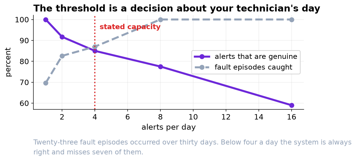
| Top 30 | 30 | 1.0 | 100.0% | 16 of 23 |
| Top 60 | 60 | 2.0 | 91.7% | 19 of 23 |
| Top 120 | 120 | 4.0 | 85.0% | 20 of 23 |
| Top 240 | 240 | 8.0 | 77.5% | 23 of 23 |
| Top 480 | 480 | 16.0 | 59.0% | 23 of 23 |
| Consensus policy | Alerts | Per day | Precision | Episodes caught |
|---|---|---|---|---|
| Any one of three | 238 | 7.9 | 55.0% | 22 of 23 |
| At least two of three | 90 | 3.0 | 72.2% | 22 of 23 |
| All three | 32 | 1.1 | 87.5% | 15 of 23 |
The two-of-three rule is recommended: it sits inside the stated capacity at 3.0 alerts per day, achieves 72.2 percent precision, and matches the best episode recall available at any budget below 8 alerts a day. Unanimity is more precise per alert and loses a third of the episodes, since the three detectors respond to different notions of outlyingness and only severe faults are extreme under all three.
Detection is not uniform across fault modes. At 4 alerts a day the best single detector catches 9 of 9 bearing-wear episodes, 8 of 8 valve drifts and 3 of 6 air leaks. The air-leak signature is the weakest and is the natural target for a second iteration.
7. Sensitivity without labels
Injection provides a sensitivity estimate that requires no labeled history. A synthetic bearing-wear episode of known amplitude is added to the clean data at a random location and the detector is refitted.
| Injected severity | Detection rate |
|---|---|
| 40% of a full episode | 42% |
| 70% | 75% |
| 100% | 100% |
This is the only sensitivity figure obtainable in production. Run on a schedule against live data it also functions as a drift monitor: a falling detection rate at fixed injected severity indicates that the reference distribution has moved and the detector requires refitting.
8. Limitations
The threshold has no statistical justification and does not require one; it is a constraint on a technician's day and moves with staffing rather than with the data.
Detection latency was not measured. Episodes are detected somewhere within their span, and whether that is early enough to prevent downstream scrap depends on the physics of each failure mode and on maintenance records this site does not keep.
The repairs assume the engineering log is complete. Three of four entries were independently recoverable from the data, but there is no way to bound how many undocumented changes remain and are being scored as anomalies. The recommended mitigation is procedural: log data-quality alerts as they are triaged.
Finally, all reported precision and recall depend on an answer key that exists only because the data were generated. In production the only available evidence is the triage outcome of each alert and the injection test in section 7, and the reporting should be built around those two from the start.