Scaling, Internal Indices, an External Criterion and a Density Method

Silhouette and stability both selected k = 2. A held-out response variable selected k = 4, which the answer key confirms at an adjusted Rand of 0.85 for k-means and 0.92 for Ward.

Data 5,693 loyalty accounts, 8 behavioral features

Methods k-means, Ward, DBSCAN; silhouette, resampling stability, external validation

Headline k = 4, of which 3 map to true segments; 55% of the base unclustered

Where this comes from

Chapter Chapter 195 · Clustering: Choosing k Honestly

Part Part XXXI · Capstone Projects: Machine Learning

Dataset capstone-clustering-choosing-k.xlsx

Notebook View the analysis

1. Sample and preparation

From 6,190 exported rows: a duplicated block of 190 removed on customer_id; 81 net-refund accounts with negative annual spend removed; 226 accounts with tenure_months = -1 (join date never migrated) removed. Analysis sample 5,693. Eight behavioral features; campaign_response, which records a campaign run the following quarter, was withheld from every clustering and used only for validation.

2. Scaling

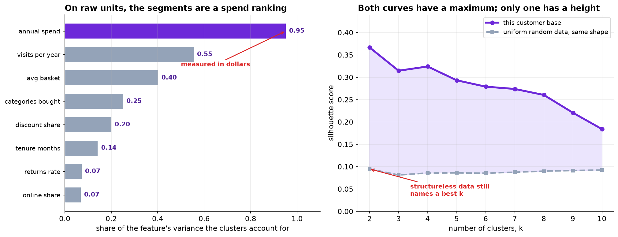
Feature standard deviations span four orders of magnitude: annual_spend at 2,134.7 against discount_share at 0.248, a ratio of about 8,600. Under a Euclidean metric this makes the partition a function of spend alone.

Table 1. Between-cluster variance as a share of total, per feature, k = 4 on unstandardized data.

Feature	Share of its variance explained by k-means on raw units
annual_spend	0.950
visits_per_year	0.554
avg_basket	0.402
categories_bought	0.251
discount_share	0.200
tenure_months	0.142
returns_rate	0.072
online_share	0.068

The resulting clusters have mean annual spends of 442, 1,405, 5,017 and 7,875 dollars and are near-identical on every behavioral rate. All subsequent analysis uses z-standardized features. That choice is itself a weighting assumption, asserting equal importance per standard deviation, and a margin-weighted alternative would produce different boundaries with no test to adjudicate between them.

3. Internal criteria

Table 2. Silhouette on a 3,000-point subsample; stability is the mean adjusted Rand between the full solution and 25 refits on 80 percent subsamples.

k	Silhouette, real	Silhouette, uniform random	Stability, real	Stability, random
2	0.3670	0.0950	0.998	0.230
3	0.3147	0.0814	0.997	0.162
4	0.3242	0.0858	0.994	0.151
5	0.2932	0.0862	0.987	0.198
6	0.2790	0.0855	0.944	0.223
7	0.2739	0.0877	0.823	0.226
10	0.1841	0.0925

Both criteria select k = 2. Both also demonstrate their own limitation. Applied to uniform random data of identical shape, silhouette still returns a maximum, at k = 2, because k-means partitions any input and silhouette merely compares partitions. What the comparison provides is a reference scale: 0.37 against 0.09 is strong evidence of structure, and that ratio is more informative than the location of either peak.

Stability separates real from structureless data decisively (0.99 against 0.15 to 0.23) and cannot separate k values within the real data, exceeding 0.98 for every k from 2 to 5. It is a test for the existence of structure, not for its cardinality.

Two panels: horizontal bars showing annual spend at 0.95 and online share at 0.07, and two silhouette curves, both with a maximum but at very different heights. — Figure 1. Left, the share of each feature's variance the raw-unit clusters account for. Right, silhouette against k for the real data and for uniform random data of the same shape.

4. External criterion

Table 3. Response to a campaign run after the observation window, never used in fitting. Base rate 0.185.

k	Min cluster response	Max cluster response	Spread	Chi-square p	ARI vs answer key
2	0.055	0.209	0.154	3.6e-27	0.321
3	0.054	0.235	0.181	2.7e-46	0.568
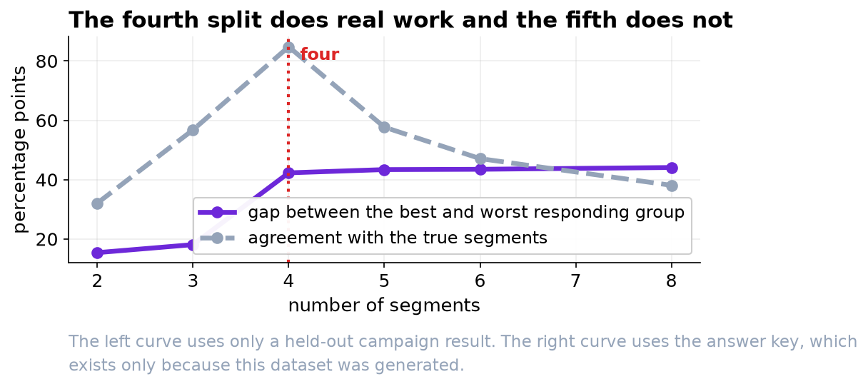
4	0.053	0.476	0.423	7.7e-179	0.848
5	0.054	0.488	0.434	4.0e-184	0.577
6	0.054	0.489	0.435	1.5e-181	0.471
8	0.054	0.495	0.441	6.1e-180	0.381

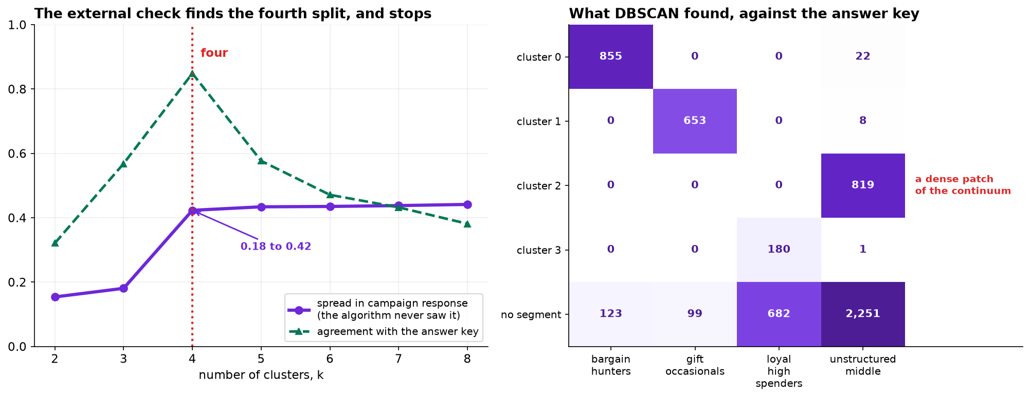
The marginal gain in separation is 0.027 for the third split, 0.242 for the fourth, and 0.011 for the fifth. The criterion selects k = 4 unambiguously, and the answer key confirms it: adjusted Rand against the true labels is 0.848 for k-means at k = 4 against 0.321 at k = 2.

Note that the chi-square p-values are uninformative here. Every partition from k = 2 upward is significant at any conventional level because n is large; the effect size is what distinguishes them. This is the standard distinction between detectable and useful, and at 5,693 accounts almost everything is detectable.

Two curves against number of segments, both turning at four. — Figure 2. The held-out campaign response spread and the agreement with the answer key, both against the number of segments. Only the first was available before the key was opened.

5. Ward and DBSCAN

Table 4. Adjusted Rand against the answer key.

k	k-means ARI	Ward ARI
2	0.321	0.316
3	0.568	0.586
4	0.848	0.924
5	0.577	0.601
6	0.471	0.527
7	0.432	0.428

Ward linkage outperforms k-means at every k from 3 to 6. The true segments differ in size (978, 862, 752 within a base of 5,693) and in dispersion, and k-means implicitly favors clusters that are comparable in both.

DBSCAN at eps = 0.9, min_samples = 25 returns four dense regions and labels 55.4 percent of accounts as noise, against a true unstructured share of 54.5 percent. On the 2,538 accounts it was willing to classify it achieves an adjusted Rand of 0.963.

Table 5. DBSCAN labels against the answer key.

DBSCAN cluster	Bargain hunters	Gift occasionals	Loyal high spenders	Unstructured middle
0	855	0	0	22
1	0	653	0	8
3	0	0	180	1
2	0	0	0	819
noise	123	99	682	2,251

Cluster 2 consists entirely of unstructured-middle accounts: a dense region of a continuum rather than a group. Its response rate of 0.126 against a base rate of 0.185 is the diagnostic that identifies it without the answer key, and it is the same external criterion used to select k, applied per cluster.

DBSCAN is highly sensitive to eps: 0.7 yields two clusters and 91.9 percent noise, 1.5 yields one cluster and 1.0 percent noise. The parameter performs the same role as k and should be selected the same way.

Two panels: the value curves peaking at four, and a table of DBSCAN clusters against true segments. — Figure 3. Left, the external check and the answer key across k. Right, what DBSCAN found set against the true segments, including the dense patch of continuum it labeled as a cluster.

6. Limitations

The standardization choice is an unfalsifiable weighting assumption and the partition is conditional on it. Sensitivity of the recommended solution to alternative weightings (margin-weighted, rank-transformed) was not assessed and would be a reasonable addition.

The external criterion validates the partition against one outcome. Segments selected to separate price promotion response carry no guarantee of separating response to service or assortment interventions, and the validation should be repeated against any new intended use.

Cluster membership is estimated from a single twelve-month window with no measurement of transition rates. Any treatment plan that assumes persistence requires a second window.

Finally, the answer key exists only because the data were generated. On observational data none of the ARI figures in sections 4 and 5 are computable, and the external criterion is the entire basis for choosing k. That is the practical situation this analysis is designed to rehearse.

← Back to Chapter 195 📓 Companion notebook 📊 Download dataset

From Statistics, Data Science and AI: A Visual Handbook by John Fisher. Every statistic, table, and figure in this report is reproduced by the companion notebook.