Where the Accuracy Came From, and Why the Point Estimate Is the Wrong Output

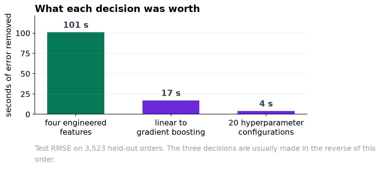
Features bought 101 seconds, model family 17, hyperparameter search 4. The learning curves then converged, and the remaining work was distributional rather than predictive.

Data 41,410 orders over 84 days, 140 restaurants

Design time-ordered split: days 0-69 train, 70-76 validate, 77-83 test

Headline test RMSE 7.882 min against a 9.898 linear baseline

Where this comes from

Chapter Chapter 193 · Gradient Boosting for Tabular Regression

Part Part XXXI · Capstone Projects: Machine Learning

Dataset capstone-gradient-boosting-regression.xlsx

Notebook View the analysis

1. Data, cleaning and design

The export held 42,520 rows. A duplicated block of 520 was removed on order_id; 384 cancellations recorded with delivery_minutes = 0 were excluded; 211 rows carrying distance_km = 999 from a GPS failure were excluded. That leaves 41,410 orders, mean 51.0 minutes, standard deviation 17.9.

The split is time-ordered rather than random, because the deployed model always predicts orders that have not occurred: days 0 to 69 for training (34,462), 70 to 76 for model selection (3,425), 77 to 83 held back (3,523). The test window was scored once.

2. Where the accuracy came from

Table 1. Test RMSE in minutes, both models at library defaults.

Feature set	Linear regression	Gradient boosting	Model family gain
Raw export columns	9.898	9.622	0.277 min
Plus four engineered features	8.017	7.946	0.071 min
Feature engineering gain	1.881 min	1.676 min

A random search over 20 hyperparameter configurations, selected on the validation window, then moved the test RMSE from 7.946 to 7.882. The three decisions therefore bought 101 seconds, 17 seconds and 4 seconds respectively.

Two details about the search matter more than its size. The 20 configurations spanned 0.272 minutes on the validation window and the top ten spanned 0.072 minutes on the test window, so among the leaders the ranking is noise; the configuration that placed tenth on validation produced the best test score (7.865). And the validation score is optimistic relative to the test score by however much the search exploited that window, so the validation figure should not be reported as model accuracy.

3. Feature ablation

Table 2. Each engineered feature removed in turn, gradient boosting at defaults.

Feature removed	Test RMSE	Cost	Derivable from present columns?
is_weekend	7.946	+0.000	Yes, from day_of_week
is_peak	7.955	+0.009	Yes, from hour_of_day
load (pending per courier)	7.958	+0.012	Yes, from its two components
rest_hist (past-only expanding median)	9.494	+1.548	No, it aggregates other rows

The pattern is structural rather than incidental. A boosted tree can split on orders_pending and couriers_available independently and approximate their ratio, and can recover the lunch and dinner peaks from hour_of_day. It has no mechanism for computing a statistic across other rows. The operational rule is to engineer what the model cannot derive from what it already holds.

rest_hist was constructed as a per-restaurant expanding median with shift(1), so each order sees only that restaurant's earlier orders. A whole-file groupby median scores marginally better on this test set and is invalid, since it conditions on future outcomes.

Bar chart of seconds of error removed by each decision. — Figure 1. The three decisions priced in seconds of test RMSE. Feature engineering returns roughly twenty-five times what the choice of model family returns.

4. Learning curve

Table 3. Random subsets of the training window, evaluated on the fixed test window.

Training orders	Train RMSE	Test RMSE	Gap
1,723	5.206	8.848	3.641
3,446	5.988	8.372	2.384
8,615	6.980	8.109	1.129
17,231	7.479	8.002	0.523
34,462	7.654	7.882	0.227

The curves converge and the final doubling of the training data reduced test RMSE by 0.121 minutes. Neither additional data of the same kind nor additional model flexibility will move this materially. The residual error is process variance, which redirects the project from point accuracy to distributional output.

5. Residual structure

Table 4. Residuals on the test window, by operating condition.

Segment	n	Bias	Residual SD
Off peak	993	-0.13	4.65
Peak	2,530	-0.07	8.83
Load under 0.8	945	-0.09	4.66
Load above 2.0	335	+0.67	11.52
Under 2 km	1,107	-0.08	6.77
Over 6 km	394	-0.30	10.35
Dry	2,780	-0.11	7.47
Heavy rain	338	+0.03	10.41

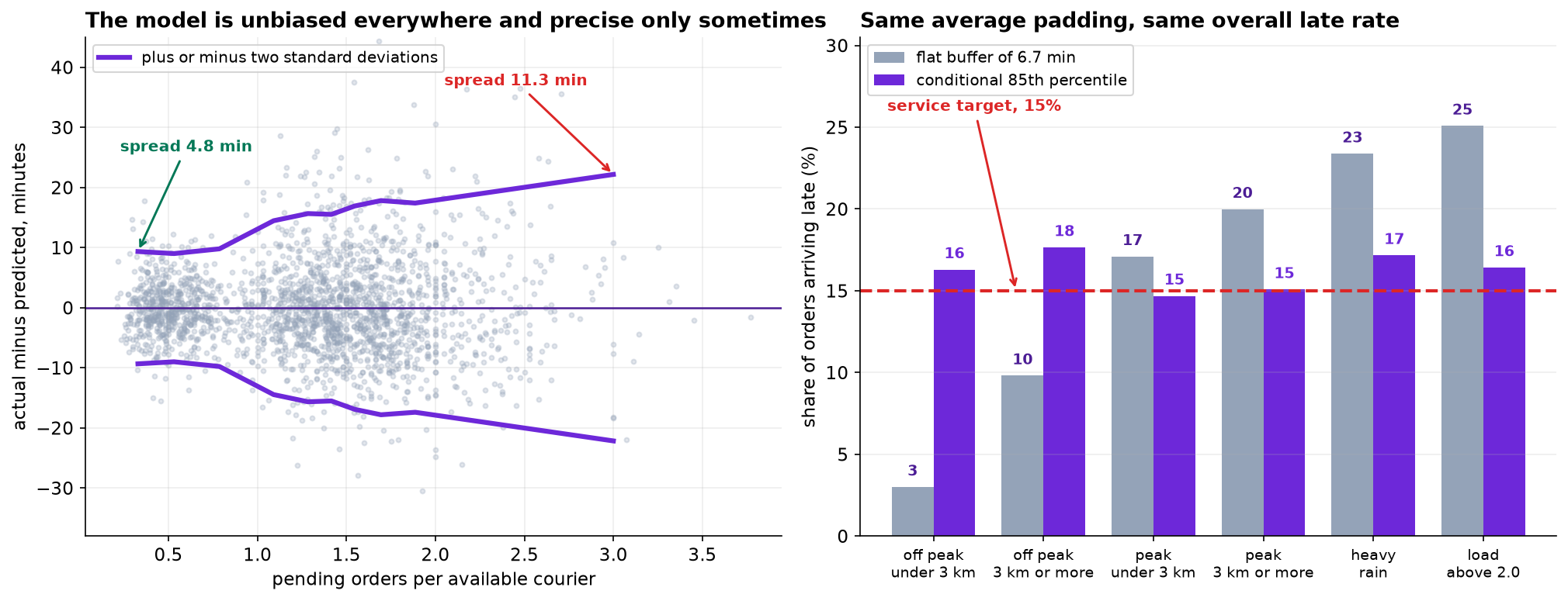
Bias is negligible throughout; the conditional standard deviation varies by a factor of about 2.5 and is predictable from features already in the model. This is the property that makes a conditional interval worth more than a constant one.

Two panels: a residual scatter with a widening envelope, and grouped bars of late rate by segment against a 15 percent target. — Figure 2. Left, prediction error against courier load, with the two-standard-deviation envelope widening from about 4.8 minutes to 11.3. Right, late rate by segment under each policy.

6. The displayed value as a quantile

The operations cost ratio is 3:1 for late against early. Under an asymmetric linear loss the minimizer is the quantile at τ = c_late/(c_late + c_early) = 0.75. Quantile-loss gradient boosting was fitted at five levels on the same features and split.

Table 5. Cost = 3 × minutes late + 1 × minutes early, averaged over test orders.

Displayed value	Late	Mean padding	Cost per order
Point prediction	46.5%	0.00	11.271
Point prediction + 8 min (current)	11.8%	8.00	11.080
Conditional 70th percentile	31.3%	2.71	9.808
Conditional 75th percentile	25.5%	3.93	9.638
Conditional 80th percentile	20.4%	5.30	9.667
Conditional 85th percentile	15.4%	6.73	10.099
Conditional 90th percentile	10.5%	8.90	11.169

The empirical minimum falls at the 75th percentile as the theory requires, 13.0 percent below the current policy. The 15 percent service target requires the 85th percentile, which costs 4.8 percent more than the cost-optimal choice. That trade is a business decision rather than a statistical one.

7. Conditional against constant padding

To isolate the value of conditioning, a constant buffer was set to the mean padding of the conditional 85th percentile (6.73 minutes), so both policies spend identical total padding.

Table 6. Share of orders arriving after the displayed time.

Segment	n	Current +8	Matched flat 6.73	Conditional 85th
Off peak, under 3 km	534	1.9%	3.0%	16.3%
Off peak, 3 km or more	459	6.8%	9.8%	17.6%
Peak, under 3 km	1,369	13.1%	17.1%	14.7%
Peak, 3 km or more	1,161	17.0%	20.0%	15.1%
Heavy rain	338	19.8%	23.4%	17.2%
Load above 2.0	335	21.8%	25.1%	16.4%
All orders	3,523	11.8%	15.0%	15.4%

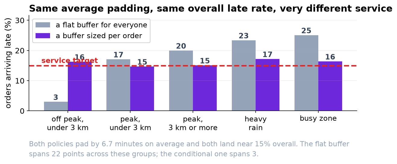
Marginal late rates are indistinguishable (15.0 against 15.4 percent). Conditional late rates differ sharply: the constant buffer spans 22.1 percentage points across these segments against 3.0 for the conditional policy. Conditional padding runs from 2.4 minutes for the easiest decile of orders to 11.8 for the hardest.

No aggregate accuracy metric detects this difference. RMSE, MAE and the marginal late rate are all effectively equal between the two policies; the divergence is entirely in the conditional coverage, and it falls systematically on the same customers.

Paired bars showing the flat buffer spanning 22 points across segments and the conditional one spanning 3. — Figure 3. Late rate by kind of order under a flat buffer and under a per-order buffer with the same average padding.

8. Limitations

The 3:1 cost ratio is a stated judgment rather than a measurement, and the optimal quantile moves with it: 0.67 at 2:1 and 0.83 at 5:1. A sensitivity table across that range should accompany any policy decision.

The model predicts under current dispatching. Displaying longer estimates on difficult orders will change customer behavior and therefore load, which changes the predictions. This feedback is not represented here, and detecting it requires a holdout that is maintained after deployment rather than a one-off evaluation.

The demand-side cost of a longer quoted time, that is, orders not placed, is absent from the dataset and from the cost function. It is the largest unmeasured quantity in the analysis and the clearest candidate for an experiment.

Eighty-four days covers a single season with no holiday peak and no restaurant turnover. The learning curve establishes that more orders of the same kind will not help; it says nothing about orders of a different kind.

← Back to Chapter 193 📓 Companion notebook 📊 Download dataset

From Statistics, Data Science and AI: A Visual Handbook by John Fisher. Every statistic, table, and figure in this report is reproduced by the companion notebook.