Imbalanced Classification: Leakage, Ranking, Calibration and Cost

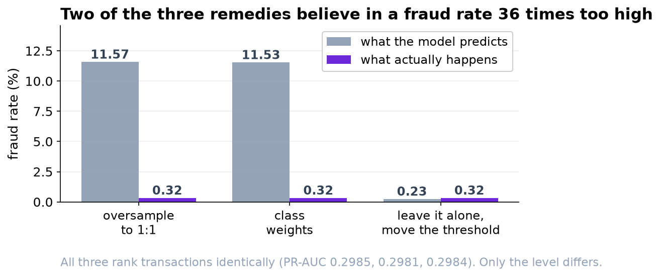
Three standard answers to a 0.32 percent positive rate rank identically to three decimal places and differ 36-fold on the level. Only one of them can be multiplied by a dollar amount.

Data 119,556 purchases after cleaning, 318 frauds (0.266%)

Design temporal split, days 1-90 train / 91-120 test

Headline PR-AUC 0.2984, cost-optimal threshold 0.0883

Where this comes from

Chapter Chapter 191 · Imbalanced Classification: Credit Card Fraud

Part Part XXXI · Capstone Projects: Machine Learning

Dataset capstone-credit-card-fraud.xlsx

Notebook View the analysis

1. Data and cleaning

The export contained 120,400 rows. Three faults were removed before any modeling: a duplicated export block (400 rows), 306 rows carrying a distance sentinel of -1 where geolocation had failed, and 138 zero-amount rows that are authorization holds rather than purchases. That leaves 119,556 transactions with 318 confirmed frauds, a rate of 0.266 percent.

Flagging nothing is 99.734 percent accurate. Accuracy is not reported again in this analysis.

2. Split and leakage

The split is temporal: days 1 to 90 for training (89,973 transactions, 223 frauds) and days 91 to 120 for testing (29,583 transactions, 95 frauds, 0.3211 percent). A random split would allow the model to learn from transactions that had not yet occurred.

Table 1. Honest features against the same model with the chargeback column added.

Feature set	ROC-AUC	PR-AUC	Reading
Honest features only	0.9604	0.2984	93× the base rate
Plus `chargeback_code_filed`	0.9997	0.9818	not available at decision time

The chargeback column is populated weeks after the transaction, once a case has been worked. It is a leak. The operational test applied throughout is whether a value would have existed, with that value, at the moment the prediction is required. Leakage does not present as an error; it presents as an implausibly good result, and a PR-AUC of 0.98 on a fraud problem is a symptom rather than a finding.

3. Model comparison

Table 2. Four models on the same temporal split. Lift is PR-AUC divided by the base rate.

Model	ROC-AUC	PR-AUC	Lift	Brier
Logistic, additive	0.9554	0.2752	86×	0.00269
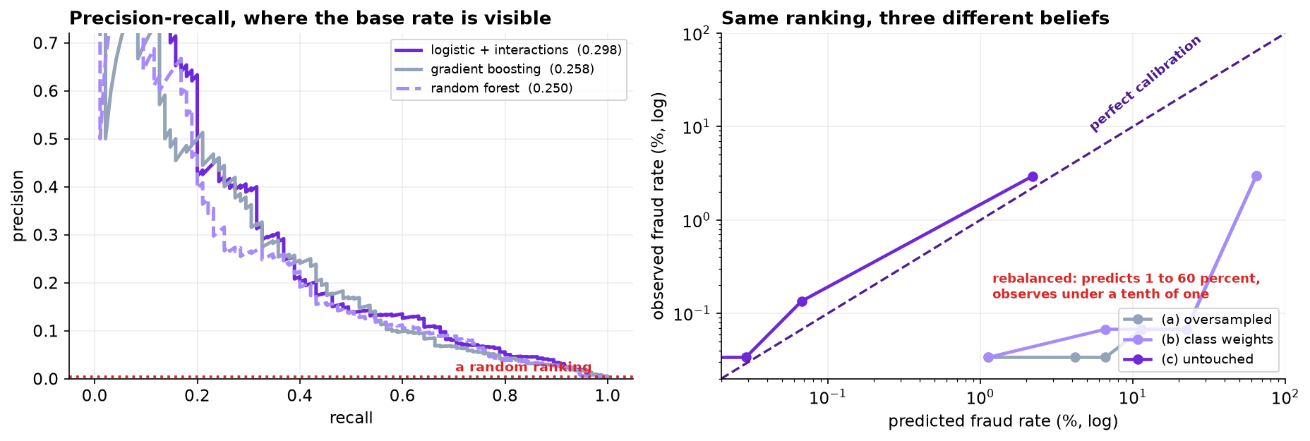
Logistic + two interactions	0.9604	0.2984	93×	0.00264
Gradient boosting	0.9565	0.2584	80×	0.00272
Random forest	0.9364	0.2496	78×	0.00285

The linear model wins, and the ensembles were not handicapped: two genuine interactions exist in the data-generating process, a new device on a card-not-present sale and a foreign merchant overnight, so there is real non-additive structure available. The ensembles cannot recover it from 223 positives. Sample size for a flexible model is counted in positives, not rows.

ROC-AUC separates the four models by 0.024 and PR-AUC by 0.049. With a false positive rate whose denominator is nearly 30,000, ROC-AUC is close to insensitive here and should not be the headline.

4. Imbalance remedies, judged on calibration

Table 3. Three imbalance remedies on the same model, split and features.

Approach	PR-AUC	Brier	Mean predicted	Observed	Ratio
(a) Random oversampling to 1:1	0.2985	0.05136	11.571%	0.3211%	36.0×
(b) Class weights	0.2981	0.05109	11.531%	0.3211%	35.9×
(c) Untouched, tuned threshold	0.2984	0.00264	0.233%	0.3211%	0.7×

The three PR-AUCs agree to three decimal places because all three fit the same model to the same information. Resampling and class weighting do not change the ordering; they change the prior the fitted model encodes, which no ranking metric can detect. The Brier scores differ by a factor of twenty, and the mean predicted probability by a factor of thirty-six.

That is decisive here because the downstream step multiplies the predicted probability by a transaction amount to form an expected loss. An inflated probability makes that product meaningless. Where a decision needs only an ordering, resampling is harmless; where it needs a probability, the remedy has removed the thing being used. Recalibration (Platt or isotonic) restores it and is a second step that is easy to forget.

Paired bars of predicted against observed fraud rate for three imbalance remedies. — Figure 1. Mean predicted fraud rate against the observed rate for each remedy. The ranking metric cannot see this difference; the Brier score and this figure can.

5. Threshold from the cost matrix

Costs supplied by operations before modeling: a false positive is $16 ($4 analyst time, $12 estimated customer cost); a false negative is the transaction amount written off plus $25 of handling. The per-transaction component of the miss cost means no fixed exchange rate between the two errors exists, which rules out Youden's index, the F1 peak and any other curve-derived rule.

Table 4. Total cost across the threshold range. The optimum is the shallow bottom of a bowl.

Threshold	Flagged	Caught	Missed	Cost, 30 days
0.0020	2,196	85	10	$35,011
0.0100	887	67	28	$16,976
0.0500	251	44	51	$10,402
0.0883	146	37	58	$9,975
0.2000	58	24	71	$11,195
0.4000	26	17	78	$11,609

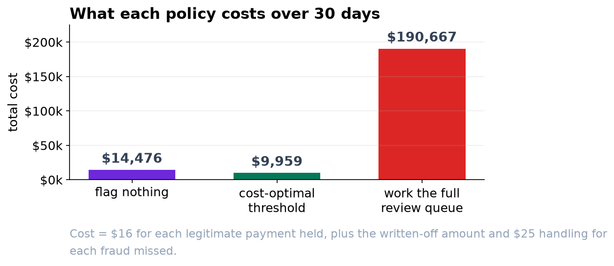
A finer sweep locates the minimum at 0.0883 with 145 flags and a cost of $9,959, against $14,476 for flagging nothing, a 31 percent reduction. The curve is shallow: the interval from roughly 0.04 to 0.15 is within a few hundred dollars of the optimum, so the policy is not sensitive to the exact threshold.

The optimal policy misses 58 of 95 frauds. This is the correct solution to the stated objective and will be read as a failure by any process measured on detection rate.

Two panels: precision-recall curves, and a log-log calibration plot showing the rebalanced models predicting far above the observed rate. — Figure 2. Left, precision-recall for the three model families against the 0.32 percent base rate. Right, calibration on log axes, where the untouched model tracks the diagonal and the two rebalanced ones do not.

6. The capacity constraint, tested

The review team's stated capacity is 400 cases a day, 12,000 over the test window. Setting the threshold to fill it (0.00012) catches 93 of 95 frauds at a cost of $190,667, which is 13 times the cost of having no model at all. Approximately 11,900 of the 12,000 reviews are of legitimate transactions at $16 each.

Capacity is therefore not the binding constraint; the unit cost of a false positive is. The cost-optimal policy uses about one percent of available capacity, which inverts the usual framing of the operational question.

Bar chart of 30-day cost: flag nothing $14,476, cost-optimal $9,959, fill the queue $190,667. — Figure 3. Total cost under the three candidate policies. Filling the review capacity is the worst of the three by an order of magnitude.

7. Limitations

The evaluation is a single temporal split, so the test estimate is one draw rather than a distribution; repeating it across rolling windows would put an interval on the 31 percent saving. The $12 customer-annoyance figure is an estimate rather than a measurement, and the threshold moves with it, though the shallowness of the curve limits how far. Fraud is adversarial and the patterns learned from days 1 to 90 will decay, so both the model and the threshold need re-measurement on a schedule.

Finally, the distribution of false positives is not uniform across customers. Travel, late-night purchases and a recently changed device all raise the predicted probability, and all three are ordinary behavior. The $16 in the cost matrix treats every false positive as equivalent, which is a modeling convenience rather than a fact.

← Back to Chapter 191 📓 Companion notebook 📊 Download dataset

From Statistics, Data Science and AI: A Visual Handbook by John Fisher. Every statistic, table, and figure in this report is reproduced by the companion notebook.