Two Natural Experiments on One Question: a Fuzzy Discontinuity and an Administrative Instrument
Identification of a scholarship effect from an eligibility threshold and from a stale allocation formula, with the assumptions each design requires and the checks each permits.
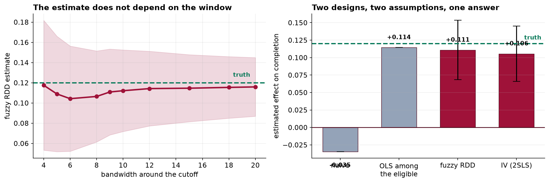
Objective. To estimate the effect of a means-tested scholarship on degree completion using designs that do not require conditional ignorability. Methods. Two identification strategies were applied to the same registry of 79,666 students. A fuzzy regression discontinuity exploited a deterministic eligibility threshold at a need index of 60, estimated by local linear regression with a triangular kernel and heteroskedasticity-robust standard errors, with the intention-to-treat jump rescaled by the discontinuity in take-up. A two-stage least squares estimator used scholarship places allocated per 100 students, set by a formula based on three-year-old enrollment counts, as an instrument for receipt among eligible students. Results. The unadjusted difference was −3.47 pp. The density of the running variable was continuous at the threshold (z = −0.59) and pre-treatment covariates were smooth (|z| < 1.7). The intention-to-treat jump was +6.94 pp (SE 1.35) against a take-up jump of 0.626 (SE 0.009), giving a fuzzy estimate of +11.09 pp (95% CI +6.84 to +15.34), stable from +10.4 to +11.6 across bandwidths of 5 to 20. The first-stage F was 2,685 and 2SLS gave +10.55 pp (95% CI +6.59 to +14.51). The true effect is +12.0 pp. Conclusion. Both designs recover the effect, and their agreement is informative because their identifying assumptions are logically independent.
1. Setting and the failure of the naive comparison
The scholarship is allocated on a means-tested need index. Recipients complete degrees at 45.31% against 48.81% among non-recipients, a difference of −3.47 pp. Since the true effect is +12.0 pp, the naive contrast is not merely attenuated but of the opposite sign, selection being both large and opposed to the treatment effect.
Conditional adjustment on recorded covariates is not pursued. The companion capstone demonstrates that in a closely analogous setting such adjustment removed under 10% of the confounding while producing a balance table that passed on every measured covariate.
2. Design A: fuzzy regression discontinuity
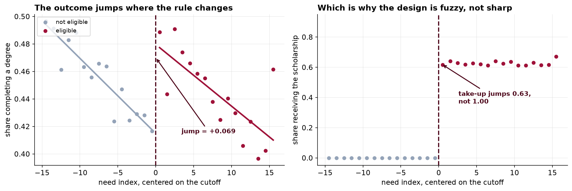
Eligibility is a deterministic step function of the need index at 60.0, and no ineligible student received an award, so assignment to eligibility is sharp while receipt is not. Identification requires only that the conditional expectation of potential outcomes be continuous in the running variable at the threshold.
| Diagnostic | Result | Interpretation |
|---|---|---|
| Density at the threshold | 749.8 below vs 727.1 above per 0.5-point bin; z = −0.59 | No evidence of sorting |
| Family income | −0.28 (SE 0.17), z = −1.63 | Continuous |
| School allocation | −0.14 (SE 0.11), z = −1.23 | Continuous |
The index is computed by an administering agency from submitted documentation rather than self-reported, which is the circumstance under which manipulation is least feasible. Where a running variable is self-reported and the threshold is publicized, this diagnostic frequently fails, and a failed density test terminates the design rather than calling for correction.
3. RDD estimation
Local linear regression with a triangular kernel was fitted separately on each side of the threshold, with heteroskedasticity-robust standard errors obtained from the weighted sandwich estimator.
| Quantity | Estimate | SE | 95% CI |
|---|---|---|---|
| Jump in completion (ITT) | +0.0694 | 0.0135 | [+0.0428, +0.0959] |
| Jump in take-up | +0.6257 | 0.0094 | — |
| Fuzzy RDD (Wald ratio) | +0.1109 | 0.0217 | [+0.0684, +0.1534] |
| Bandwidth | n | Fuzzy estimate | 95% CI |
|---|---|---|---|
| ±5 | 14,599 | +0.1089 | [+0.0518, +0.1660] |
| ±6 | 17,405 | +0.1043 | [+0.0522, +0.1563] |
| ±8 | 22,996 | +0.1064 | [+0.0614, +0.1515] |
| ±9 | 25,676 | +0.1109 | [+0.0684, +0.1534] |
| ±12 | 33,580 | +0.1142 | [+0.0773, +0.1512] |
| ±15 | 40,867 | +0.1146 | [+0.0814, +0.1478] |
| ±20 | 51,519 | +0.1159 | [+0.0869, +0.1449] |
The Wald ratio is an instrumental variables estimator in which the instrument is the indicator of crossing the threshold. This should be stated explicitly, since it clarifies both the interpretation of the estimand and the sense in which the two designs presented here are relatives rather than independent methods. What distinguishes them is not the estimator but the exclusion restriction each requires.
A note on efficiency. The registry contains 79,666 records and the reported specification uses 25,676 of them, weighted toward the threshold. The design purchases credibility with precision, and the resulting interval spans 8.5 percentage points.
4. Design B: instrumental variables
Scholarship places are allocated to high schools by a formula computed from enrollment counts three years prior. The instrument is places per 100 students. Estimation is restricted to eligible students, since receipt is identically zero otherwise, and the need index is included as a control.
| Assumption | Testable | Evidence |
|---|---|---|
| Relevance | Yes | First-stage coefficient +0.0351 (SE 0.0007), t = 51.8, F = 2,685 |
| Monotonicity | Partially | Take-up rises monotonically across all five allocation quintiles, 0.418 to 0.820 |
| Exclusion | No | Argued from the staleness of the formula; unfalsifiable |
The first-stage F exceeds the conventional threshold of 10 by more than two orders of magnitude. This settles relevance alone. A strong first stage is routinely presented as evidence of instrument validity and is nothing of the kind; it establishes only that the instrument shifts the treatment.
The exclusion restriction requires that the allocation affect completion solely through receipt. The supporting argument is that the formula uses enrollment counts predating the cohort by three years and therefore carries no information about it. The principal objection is that lagged enrollment may proxy for neighborhood characteristics correlated with completion. The falsification evidence available is that the allocation is continuous at the eligibility threshold and unrelated to family income there. This is supportive and not dispositive, and the assumption should be reported as an assumption.
| Estimator | Estimate | SE | 95% CI |
|---|---|---|---|
| 2SLS (LATE) | +0.1055 | 0.0202 | [+0.0659, +0.1451] |
| OLS, eligible sample | +0.1145 | — | — |
OLS on the eligible sample returns +0.1145, close to both the IV estimate and the truth. This is not coincidental: conditional on eligibility, receipt is largely determined by the school's allocation, which is plausibly exogenous, so little confounding remains within that subgroup. The observation is reported rather than suppressed because it would be misleading to present the instrument as having rescued an analysis that a subgroup restriction largely handled. The instrument's contribution is that its validity does not depend on that circumstance holding.
5. Comparison
| Estimator | Estimate | 95% CI | Identifying assumption |
|---|---|---|---|
| Naive | −0.0347 | — | Conditional ignorability, unconditionally |
| OLS, eligible | +0.1145 | — | Conditional ignorability within the eligible |
| Fuzzy RDD | +0.1109 | [+0.0684, +0.1534] | Continuity of potential outcomes at need = 60 |
| 2SLS | +0.1055 | [+0.0659, +0.1451] | Exclusion of the allocation from the outcome equation |
| Truth | +0.1200 | — | — |
Neither identifying assumption implies the other. Continuity at a threshold is a statement about the local behavior of potential outcomes in the running variable; the exclusion restriction is a statement about a school-level administrative variable. For the two estimates to coincide under joint failure, both assumptions would need to be violated in unrelated directions and by comparable magnitudes. The concordance is therefore informative, in contrast to the agreement between matching and weighting estimators in the companion capstone, which share an identifying assumption and fail jointly by construction.
6. Estimands
Both estimates are local and their localities differ. The RDD identifies an effect for students whose need index lies near 60 and whose receipt was determined by eligibility. The 2SLS estimate identifies a local average treatment effect over compliers: students whose receipt was shifted by their school's allocation. Neither is the average effect among all recipients, and neither extrapolates to students who would become eligible under a lower threshold. Where the policy question concerns expansion, the relevant population is precisely the one on which neither design carries information.
7. Discussion
The comparison with the companion capstone is the substantive point. There, adjustment on a rich set of pre-treatment covariates achieved excellent balance and removed under 10% of the bias, because the covariates were nearly orthogonal to the selection mechanism. Here, no covariate is used for identification at all. The estimates derive from an administrative threshold and an obsolete funding formula, neither of which any student chose, and both recover the truth.
This is not an argument that natural experiments are superior in general. They are unavailable in most settings, they answer narrower questions than they appear to, and their assumptions are untestable in a different way rather than in a lesser way. The argument is narrower: when such variation exists it should be sought before adjustment is attempted, because a credible design answers a small question reliably while adjustment answers a large question at unknown risk.
A limitation of the present analysis is that bandwidths were selected by inspection across a stated range rather than by a data-driven rule. Contemporary practice would report an MSE-optimal bandwidth with bias-corrected robust intervals. The range is presented here in preference to a single automated choice for transparency, and the estimate's stability across it is the relevant evidence either way.
8. Conclusion
A means-tested scholarship raises degree completion by approximately 11 percentage points. A fuzzy regression discontinuity at the eligibility threshold gives +11.09 pp (95% CI +6.84 to +15.34) and an instrumental variables estimate using an administrative allocation formula gives +10.55 pp (95% CI +6.59 to +14.51), against a true value of +12.0 pp. The unadjusted comparison gives −3.47 pp. The two designs rest on logically independent assumptions, which is the basis on which their agreement is treated as evidence.
References
- Thistlethwaite, D. L., & Campbell, D. T. (1960). Regression-discontinuity analysis: an alternative to the ex post facto experiment. Journal of Educational Psychology, 51(6), 309–317.
- Imbens, G. W., & Lemieux, T. (2008). Regression discontinuity designs: a guide to practice. Journal of Econometrics, 142(2), 615–635.
- Lee, D. S., & Lemieux, T. (2010). Regression discontinuity designs in economics. Journal of Economic Literature, 48(2), 281–355.
- Calonico, S., Cattaneo, M. D., & Titiunik, R. (2014). Robust nonparametric confidence intervals for regression-discontinuity designs. Econometrica, 82(6), 2295–2326.
- McCrary, J. (2008). Manipulation of the running variable in the regression discontinuity design: a density test. Journal of Econometrics, 142(2), 698–714.
- Imbens, G. W., & Angrist, J. D. (1994). Identification and estimation of local average treatment effects. Econometrica, 62(2), 467–475.
- Angrist, J. D., Imbens, G. W., & Rubin, D. B. (1996). Identification of causal effects using instrumental variables. Journal of the American Statistical Association, 91(434), 444–455.
- Angrist, J. D., & Pischke, J.-S. (2009). Mostly Harmless Econometrics. Princeton University Press.
- Stock, J. H., & Yogo, M. (2005). Testing for weak instruments in linear IV regression. In Identification and Inference for Econometric Models. Cambridge University Press.
Reproducibility
The dataset (capstone-regression-discontinuity-and-iv.xlsx) contains the registry export with its data-quality faults intact, the analysis plan as written before outcome linkage, and the generating parameters. An executable notebook accompanies the chapter and reproduces every estimate, table and figure, implementing kernel-weighted local linear regression, its robust variance and two-stage least squares directly rather than through a specialized package. Analyses use NumPy, pandas, statsmodels and Matplotlib.