A Two-Stage Cluster Sample of Schools: Design Effect, Effective Sample Size and Interval Coverage
Variance decomposition, three standard-error estimators, and a coverage experiment on a synthetic population.
Objective. To estimate mean sixth-grade reading achievement across a district, and to quantify the precision consequences of the cluster design the sampling frame required. Methods. No enumeration of students exists; a complete list of 120 schools does. A two-stage design drew 24 schools by simple random sampling and 25 students within each, yielding n = 597 after cleaning. The intra-class correlation was estimated from a one-way variance decomposition and the design effect as 1 + (m − 1)ρ. Three standard errors are compared: naive, design-effect corrected, and the ultimate-cluster estimator. Interval coverage was assessed over 1,000 replicate samples drawn from a synthetic population matched to the estimated variance components. Results. Between-school and within-school mean squares were 2,256.2 and 244.7, giving ρ = 0.2484 (population value 0.2225) and a design effect of 6.93. Effective sample size was 86.1. The naive standard error (0.7348) understated the corrected value (1.9343) by a factor of 2.63; the ultimate-cluster estimator agreed closely (1.9420). Nominal 95% intervals ignoring the design achieved 56.9% coverage against 96.6% for the corrected interval. Conclusions. The design effect is the dominant feature of this study. Reallocating the same number of assessments across more schools would raise the effective sample size from 86 to approximately 301.
1. Introduction
Cluster sampling is adopted when no frame of elementary units exists, or when the cost of reaching a dispersed sample is prohibitive. Both conditions hold here. The resulting design is administratively straightforward and statistically expensive, and the expense is incurred in a quantity that standard software does not report by default: the variance of the estimator is inflated by a factor that depends on how much the elementary units within a cluster resemble one another.
The consequence is not a small correction. At the intra-class correlation observed in educational achievement data, and at the cluster sizes ordinarily used, the inflation factor is commonly between three and ten. An analysis that treats a cluster sample as a simple random sample therefore reports a standard error understated by a factor of two or three, and a confidence interval whose nominal coverage bears little relation to its actual coverage. Section 5 quantifies the latter directly.
2. Design and data
| Element | Specification |
|---|---|
| Target population | 8,184 sixth-grade students in 120 schools |
| Frame | No student-level frame exists. A complete school-level frame with enrollment counts does |
| Stage 1 | 24 schools by simple random sampling without replacement |
| Stage 2 | 25 students by simple random sampling within each selected school |
| Realized n | 597 students after removing duplicates, one out-of-range score and two absentees |
| Outcome | District reading assessment, 0–100; the standard is defined in advance as 65 |
Cleaning removed two duplicate records, one score of 155 on a 0–100 instrument, and two students absent on the assessment day. The last of these leaves the clusters marginally unbalanced (23 of 24 schools contribute 25 students, one contributes 24), which the estimators below accommodate through the realized mean cluster size.
3. Variance decomposition and the design effect
| Quantity | Value | Definition |
|---|---|---|
| Mean square between | 2,256.20 | Variation of school means about the grand mean |
| Mean square within | 244.71 | Variation of students about their own school mean |
| Intra-class correlation | 0.2484 | (MSB − MSW) / (MSB + (m − 1)MSW) |
| Population ρ | 0.2225 | Known here; unavailable in applied work |
| Mean cluster size | 24.88 | Realized, allowing for the two absentees |
| Design effect | 6.930 | 1 + (m − 1)ρ |
| Effective sample size | 86.1 | n / design effect |
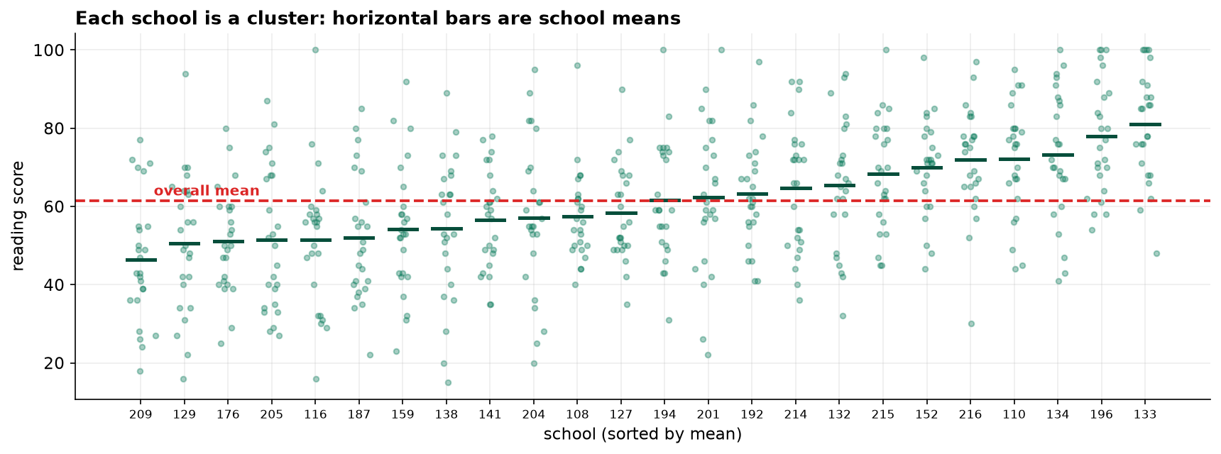
An intra-class correlation of 0.25 is unremarkable for educational achievement, where intake composition, teaching and neighborhood covary at the institution level. Its practical import is entirely a function of cluster size: at m = 25 the multiplier is 6.93, so the 597 assessments carry the information of 86 independently drawn students. Approximately 511 assessments contributed negligibly to the precision of the district estimate.
4. Estimation
| Estimator | SE | 95% CI | Covers true mean | Basis |
|---|---|---|---|---|
| Naive (independence) | 0.7348 | [59.97, 62.85] | Yes | s / √n, ignores the design |
| Design-effect corrected | 1.9343 | [57.61, 65.20] | Yes | naive × √deff |
| Ultimate cluster | 1.9420 | [57.60, 65.21] | Yes | SD of the 24 school means / √24 |
The two design-aware estimators agree to within 0.0077, which is reassuring given that they proceed differently. The ultimate-cluster estimator discards the within-cluster information entirely and treats the 24 school means as the sample, an approach that requires no assumption about equal cluster sizes or a constant intra-class correlation. Their agreement supports the substantive claim that this study carries 24 independent units of information rather than 597.
The naive estimator understates the standard error by a factor of 2.63. That it nonetheless produces an interval covering the true value in this realization is a property of this draw and not of the method.
5. Interval coverage
A single realization cannot establish the operating characteristics of an interval procedure. A synthetic population was therefore constructed with between-school and within-school standard deviations set to the values estimated in Section 3, and the sampling design was replicated 1,000 times against it.
| Interval | Nominal coverage | Actual coverage | Actual error rate |
|---|---|---|---|
| Naive (independence) | 95% | 56.9% | 43.1% |
| Design-effect corrected | 95% | 96.6% | 3.4% |
The naive procedure fails to cover the target parameter in roughly two replications in five, while reporting a 5 percent error rate. The discrepancy is a factor of approximately eight. This is the substantive finding of the report: the failure is not one of point estimation, which is unbiased, but of stated precision, and it is invisible to any diagnostic computed from a single sample.
6. Design optimization at fixed cost
| Design | Design effect | Effective n | Relative precision |
|---|---|---|---|
| 12 schools × 50 students | 13.17 | 45.6 | 0.73× |
| 24 schools × 25 students | 6.96 | 86.2 | 1.00× |
| 40 schools × 15 students | 4.48 | 134.0 | 1.25× |
| 60 schools × 10 students | 3.24 | 185.5 | 1.47× |
| 120 schools × 5 students | 1.99 | 301.0 | 1.87× |
Effective sample size is monotone decreasing in cluster size. Reallocating the same 597 assessments to 60 schools of 10 students would raise the effective n from 86 to 185, and to 120 schools of 5 students would raise it to 301. The marginal statistical value of an additional cluster greatly exceeds that of an additional unit within an existing cluster, and the optimal allocation under a cost model depends on the ratio of per-cluster to per-unit cost. That calculation belongs in the design phase.
7. The binary outcome
| Quantity | Value |
|---|---|
| Proportion meeting the standard | 43.55% (260 of 597) |
| True population proportion | 41.41% |
| Intra-class correlation | 0.1962 |
| Design effect | 5.68 |
| Naive Wilson 95% CI | [39.63%, 47.56%] |
| Cluster-corrected 95% CI | [34.07%, 53.03%] |
Binary outcomes cluster in the same manner as continuous ones. Wilson, Agresti-Coull and Clopper-Pearson intervals all presuppose independent Bernoulli trials, and none carries a warning when that presupposition fails. The corrected interval here is 2.4 times the width of the naive one.
8. Discussion
Three points generalize. First, the primary sampling unit must be identified before any standard error is computed, and it is a property of the design rather than of the data file. Nothing in the dataset marks school_id as special; only the sampling plan does. Second, the design effect belongs in the planning stage, where it determines the allocation, rather than the analysis stage, where it only quantifies a loss already incurred. Third, coverage rather than point bias is the failure mode: the naive estimator is unbiased and its interval is nonetheless wrong most of the time it is wrong.
Two ethical considerations attach specifically to cluster designs. Consent operates at the cluster level, so a single institutional refusal removes an entire cluster, and institutions do not decline at random. And because school-level means are visible in the data, there is a standing temptation to report them; each rests on 25 students, and a ranking constructed from them would be substantially noise with material consequences attached to it. The design supports a district estimate and does not support institutional comparison.
A design limitation is disclosed rather than corrected. Sampling a fixed 25 students per school gives students in small schools a higher selection probability than students in large ones. A fully design-based analysis would carry inverse-probability weights; this analysis does not, and the resulting estimate is therefore self-weighting only to the extent that school size is unrelated to achievement.
9. Conclusion
Mean sixth-grade reading achievement in the district is estimated at 61.41 (95% CI 57.61 to 65.20, design effect 6.93, effective n = 86). The naive standard error is understated by a factor of 2.63 and the corresponding interval attains 56.9% coverage against a nominal 95%. Reallocating the same assessment budget across more schools with fewer students in each would raise the effective sample size by a factor of up to 3.5.
References
- Kish, L. (1965). Survey Sampling. Wiley.
- Cochran, W. G. (1977). Sampling Techniques (3rd ed.). Wiley.
- Kish, L. (1995). Methods for design effects. Journal of Official Statistics, 11(1), 55–77.
- Donner, A., & Klar, N. (2000). Design and Analysis of Cluster Randomization Trials in Health Research. Arnold.
- Hedges, L. V., & Hedberg, E. C. (2007). Intraclass correlation values for planning group-randomized trials in education. Educational Evaluation and Policy Analysis, 29(1), 60–87.
- Snijders, T. A. B., & Bosker, R. J. (2012). Multilevel Analysis (2nd ed.). Sage.
- Valliant, R., Dever, J. A., & Kreuter, F. (2018). Practical Tools for Designing and Weighting Survey Samples (2nd ed.). Springer.
Reproducibility
The dataset (capstone-cluster-sampling-schools.xlsx), containing the sampled students with cluster identifiers, the school frame, the sampling plan and the enumerated population values, accompanies the chapter together with an executable notebook reproducing every statistic, table, figure and the coverage experiment. Analyses use NumPy, pandas, SciPy, statsmodels and Matplotlib.