A Stratified National Customer Survey: Design, Non-Response and Post-Stratification
Neyman allocation, weighting to population margins, and a validation against the known population value.
Objective. To estimate the proportion of customers who would recommend the service, to a specified precision, and to quantify the contribution of non-response to the resulting estimate. Methods. A stratified random sample was drawn from a frame of 55,462 contactable customers within a population of 60,000. Region formed the stratum, with Neyman allocation using pilot within-stratum standard deviations. 1,200 customers were invited and 739 responded (61.6%). Region and age band were carried from the frame for responders and non-responders alike, permitting post-stratification to population margins. Effective sample size follows Kish. Results. Response propensity varied by 50 percentage points across age bands (34.0% for 18-34, 83.5% for 55+), producing a respondent pool over-representing the 55+ band by 13.4 points. The unweighted estimate was 63.46% (95% CI 59.93 to 66.86); the post-stratified estimate was 60.64% (95% CI 56.77 to 64.51), with design effect 1.21 and effective n = 612. Against the known population value of 58.41%, the unweighted interval excluded the true value while the weighted interval covered it; weighting removed 56% of the bias. Conclusions. Differential non-response on a frame variable produced a biased estimate whose nominal precision was unaffected. Post-stratification substantially but incompletely corrected it; the residual is attributable to coverage error and to non-response on the outcome itself, neither of which is addressable by weighting.
1. Introduction
Survey estimates are conventionally reported with a margin of error derived from the sampling variance alone. That quantity addresses one component of total survey error and is silent on the remaining three: coverage, non-response and measurement. The omission is not merely incomplete but potentially misleading, since none of the three diminishes with sample size, and a design that increases n while leaving them unaddressed produces an estimate that is more precisely wrong.
This study was constructed so that the point can be demonstrated rather than asserted. The population is fully enumerated, so the target parameter is known exactly. The analysis proceeds as it would in practice, and the resulting estimates are then compared against the true value. The comparison is unavailable in applied work and is reported here for its instructional value.
2. Design
| Element | Specification |
|---|---|
| Target population | All 60,000 active retail customers on the register at the study date |
| Sampling frame | 55,462 customers holding a usable contact record (92.4% coverage) |
| Stratification | Region (4 strata), selected for reportability and for between-stratum variation |
| Allocation | Neyman: proportional to NhSh, using pilot standard deviations |
| Target precision | ± 3.0 percentage points at 95% confidence on a proportion near 0.5 |
| Invitations | 1,200 against the 1,616 implied by the target and expected response rate |
| Region | Population | Frame | Excluded | Pilot SD | Proportional | Neyman |
|---|---|---|---|---|---|---|
| Northeast | 18,000 | 16,694 | 7.3% | 1.25 | 360 | 353 |
| Midwest | 14,000 | 13,032 | 6.9% | 1.35 | 280 | 297 |
| South | 20,000 | 18,951 | 5.2% | 1.05 | 400 | 330 |
| West | 8,000 | 6,785 | 15.2% | 1.75 | 160 | 220 |
Two features of the design warrant comment. First, allocation is optimal rather than proportional: the West receives 18.3% of invitations against a population share of 13.3%, because its within-stratum standard deviation (1.75) is two thirds larger than the South's (1.05). Optimal allocation minimizes the variance of the overall estimate for a given cost, at the price of unequal selection probabilities that must be reversed analytically.
Second, the invitation count was constrained by budget below the level implied by the precision requirement. Achieving 1,050 usable responses at an anticipated 65% response rate requires approximately 1,616 invitations; 1,200 were issued. The shortfall was recorded in the sampling plan in advance, together with its consequence, a realized margin of error near 3.5 rather than 3.0 percentage points.
3. Non-response
| Stratum or band | Invited | Responded | Rate |
|---|---|---|---|
| Northeast | 353 | 235 | 66.6% |
| Midwest | 297 | 182 | 61.3% |
| South | 330 | 227 | 68.8% |
| West | 220 | 95 | 43.2% |
| Age 18-34 | 335 | 114 | 34.0% |
| Age 35-54 | 472 | 297 | 62.9% |
| Age 55+ | 393 | 328 | 83.5% |
| Age band | Population share | Respondent share | Difference |
|---|---|---|---|
| 18-34 | 29.6% | 15.4% | -14.2 pp |
| 35-54 | 39.4% | 40.2% | +0.8 pp |
| 55+ | 31.0% | 44.4% | +13.4 pp |
The distinction between the two tables above is the operative one. Region was anticipated in the design and partially offset by allocation. Age was not, and produced an imbalance of 13 to 14 percentage points in both tails of the distribution. Because age band was carried from the frame rather than elicited on the instrument, it is known for the 461 non-responders as well as the 739 responders, and can therefore serve as a weighting margin.
4. Estimation
| Quantity | Unweighted | Post-stratified |
|---|---|---|
| Point estimate | 63.46% | 60.64% |
| Standard error | 0.0177 | 0.0197 |
| 95% confidence interval | [59.93%, 66.86%] | [56.77%, 64.51%] |
| Margin of error | ± 3.47 pp | ± 3.87 pp |
| Effective sample size | 739 | 612.4 |
| Design effect | 1.00 | 1.21 |
| Weight range | — | 0.62 to 2.83 (4.6×) |
Post-stratification reduced the estimate by 2.82 percentage points and increased the standard error by 11.5%. The latter is the expected consequence of unequal weighting: the Kish effective sample size falls from 739 to 612, a design effect of 1.21. Weighting therefore trades bias against variance, and the validation below establishes that the trade was favorable.
5. Validation against the known population value
| Estimator | Estimate | 95% CI | Error | Covers true value |
|---|---|---|---|---|
| Unweighted | 63.46% | [59.93%, 66.86%] | +5.05 pp | No |
| Post-stratified | 60.64% | [56.77%, 64.51%] | +2.23 pp | Yes |
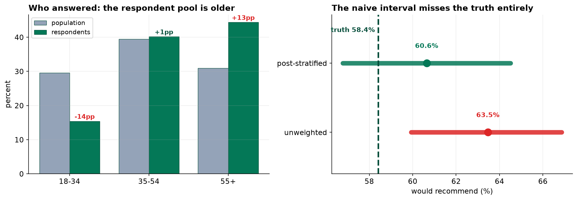
The unweighted interval excludes the true value. This is the substantive result of the exercise: the estimator was biased by 5.05 percentage points while reporting a margin of error of 3.47, and no diagnostic computed from the respondent data alone would have revealed it. Nominal precision was unaffected by the bias, which is precisely why precision is not evidence of accuracy.
The post-stratified interval covers the true value. Weighting removed 56% of the bias at a cost of 11% in standard error.
6. Residual bias
A residual of +2.23 percentage points remains after weighting, attributable to two sources that post-stratification cannot address.
Coverage. 4,538 customers (7.6%) held no usable contact record and had zero probability of selection. Exclusion is differential: 15.2% of customers in the West are absent from the frame against 5.2% in the South, and the excluded group skews young. Weighting operates within the realized sample and cannot restore units that were never eligible for selection.
Non-response on the outcome. Within age bands, response propensity increased with satisfaction, and satisfaction is associated with the recommend outcome. Adjustment would require satisfaction as a weighting margin, which is unavailable: it is observed only among responders, and the responder distribution is precisely what is in question. This is a general property rather than a limitation of this study. A variable elicited on the instrument cannot serve as an adjustment for non-response to that instrument.
7. Stratum estimates
| Region | n | Weighted estimate | 95% CI | True value | Covers |
|---|---|---|---|---|---|
| Northeast | 235 | 63.9% | [57.4%, 70.4%] | 58.7% | Yes |
| Midwest | 182 | 57.2% | [49.3%, 65.1%] | 55.5% | Yes |
| South | 227 | 63.8% | [56.7%, 70.9%] | 66.2% | Yes |
| West | 95 | 51.4% | [40.7%, 62.1%] | 43.5% | Yes |
All four stratum intervals cover their true values, as a correctly specified procedure should deliver. The intervals are nevertheless wide: the West rests on 95 responses and spans 21.4 percentage points. Stratum-level estimates from this design support description but not ranking, and any comparative claim between regions would require a substantially larger allocation.
8. Discussion
Three conclusions generalize beyond this dataset. First, differential non-response on a variable related to the outcome biases the estimate without affecting its nominal precision, so a narrow confidence interval provides no assurance against it. Second, correction is possible only for variables observed on the full invited sample, which makes the decision to carry auxiliary variables from the frame rather than eliciting them on the instrument a consequential design choice rather than an administrative convenience. Third, weighting is a bias-variance trade and should be reported as such, with the weight range and effective sample size disclosed alongside the estimate.
The response rate itself warrants specific comment. At 61.6% this survey would be regarded as satisfactory by conventional standards, and the unweighted estimate was nonetheless biased by more than five percentage points. Conversely a lower rate with response propensity unrelated to the outcome would have produced an unbiased estimate. The response rate is therefore uninformative in isolation, and reporting it without an accompanying composition analysis conveys little.
Ethical considerations attach to the coverage shortfall. Customers absent from the frame are disproportionately young and disproportionately located in the West. Where survey findings inform resource allocation, systematic exclusion of a demographic from the evidence base compounds rather than merely reflects existing differences in access, and the exclusion should be reported in the body of any resulting document rather than in an appendix.
9. Conclusion
The post-stratified estimate of the recommend proportion is 60.64% (95% CI 56.77 to 64.51, effective n = 612, design effect 1.21). The unweighted estimate of 63.46% is biased upward by 5.05 percentage points by differential non-response across age bands, and its confidence interval excludes the true population value. A residual bias of +2.23 points remains, attributable to frame under-coverage and to response propensity associated with the outcome, neither of which is correctable by weighting.
References
- Neyman, J. (1934). On the two different aspects of the representative method. Journal of the Royal Statistical Society, 97(4), 558–625.
- Kish, L. (1965). Survey Sampling. Wiley.
- Cochran, W. G. (1977). Sampling Techniques (3rd ed.). Wiley.
- Groves, R. M. (2006). Nonresponse rates and nonresponse bias in household surveys. Public Opinion Quarterly, 70(5), 646–675.
- Groves, R. M., & Peytcheva, E. (2008). The impact of nonresponse rates on nonresponse bias: a meta-analysis. Public Opinion Quarterly, 72(2), 167–189.
- Little, R. J. A., & Vartivarian, S. (2005). Does weighting for nonresponse increase the variance of survey means? Survey Methodology, 31(2), 161–168.
- Valliant, R., Dever, J. A., & Kreuter, F. (2018). Practical Tools for Designing and Weighting Survey Samples (2nd ed.). Springer.
Reproducibility
The dataset (capstone-stratified-customer-survey.xlsx), which includes the sampling plan, the instrument, the full invited sample with response indicators, the population margins and the enumerated population values, accompanies the chapter together with an executable notebook reproducing every statistic, table and figure. Analyses use NumPy, pandas, SciPy, statsmodels and Matplotlib.