Signup Rates Against a Target and Between Two Campaigns
One-sample and two-sample tests of proportions, with exact confirmation.
Keywords: proportion z-test; Wilson interval; exact binomial test; absolute versus relative risk; statistical power; A/B testing.
1. Introduction
Binary outcomes summarized as proportions are the dominant outcome type in product experimentation. Although a proportion is the mean of an indicator variable, its sampling variability is governed by the binomial, so the standard error is a function of the proportion itself rather than a separately estimated dispersion. Two distinct comparisons arise: against a fixed externally specified value, and between two independently estimated proportions.
The hypotheses are, for the one-sample comparison, H₀: πᵤ = 0.07 against a two-sided alternative; and for the two-sample comparison, H₀: πᵥ = πᵤ against a two-sided alternative. Both are evaluated at α = 0.05.
2. Data
Records comprise one row per visitor with a campaign label and a binary signup indicator. Duplicate rows and records with an unrecorded outcome were removed; missing outcomes were not imputed as non-signups, since the mechanism is unknown and such imputation would bias the rates downward.
| Step | Rule | Result |
|---|---|---|
| Raw export | — | 3,002 rows |
| De-duplication | drop duplicate rows | 3,000 rows |
| Outcome recorded | drop rows with missing signed_up | 2,998 rows |
| Campaign | Signups | Visitors | Rate | Successes / failures |
|---|---|---|---|---|
| A | 113 | 1,499 | 0.0754 (7.54%) | 113 / 1,386 |
| B | 171 | 1,499 | 0.1141 (11.41%) | 171 / 1,328 |
3. Methods
The normal approximation to the binomial requires a sufficient count of both outcomes, conventionally at least ten of each; both campaigns exceed this by two orders of magnitude. For the one-sample test the standard error was computed under the null proportion, which is the appropriate variance specification when testing against a fixed value. The Wilson score interval was preferred to the Wald interval for the single proportion because of its superior coverage. An exact binomial test was computed as a specification check on the approximation. The two-sample comparison used a pooled-variance z-test with an unpooled (Wald) interval for the difference. Analyses used statsmodels and SciPy in Python 3.
4. Results
| Comparison | Statistic | p | Interval | Decision |
|---|---|---|---|---|
| A vs target (one-sample) | z = 0.817 | 0.4140 | 95% Wilson [0.0631, 0.0899] | retain H₀ |
| A vs target (exact binomial) | — | 0.4177 | — | retain H₀ |
| B vs A (two-sample) | z = 3.617 | 2.98e-04 | 95% CI for difference [0.0178, 0.0596] | reject H₀ |
The one-sample comparison is inconclusive. The observed rate exceeds the target by 0.54 percentage points, but the Wilson interval [6.31%, 8.99%] contains 7%, so the data do not discriminate between a true rate above and below target. The exact binomial test returns a materially identical p-value, confirming that the retention is not an artifact of the approximation.
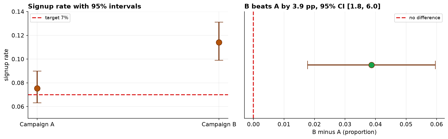
The two-sample comparison rejects decisively. The absolute risk difference is 3.87 percentage points (95% CI [1.78, 5.96]), corresponding to a relative lift of 51.3% and approximately 387 additional signups per 10,000 visitors. The contrast between the two analyses is instructive: an identical sample size resolves a 3.87-point difference easily while leaving a 0.54-point difference unresolved, illustrating that detectability is governed by effect magnitude relative to standard error rather than by sample size alone.
5. Precision, and what the design could detect
| Quantity | Value |
|---|---|
| Observed rate, campaign A | 7.54%, 95% CI 6.31% to 8.99% |
| Margin of error | ± 1.34 percentage points |
| Minimum detectable difference, 80% power | 1.96 pp (true rate 8.96%) |
| Minimum detectable difference, 90% power | 2.29 pp (true rate 9.29%) |
| Sample required for the observed 0.54 pp difference | approximately 18,000 visitors |
The one-sample comparison against the 7 percent target returned p = 0.41, and the confidence interval contains the target. Neither result constitutes evidence that the target was met. The relevant question is the sensitivity of the design, and it is answered by the detectable-effect analysis rather than by the test.
At the realized sample size the study had 80 percent power only against true rates of approximately 8.96 percent or higher. The observed rate of 7.54 percent lies within the region in which the design had low probability of detecting a departure, so the non-rejection is attributable to insufficient sensitivity and not to the absence of a difference.
Confirming a difference of the magnitude observed would require of the order of 18,000 visitors, approximately twelve times the realized sample. This is a design parameter to be fixed in advance of the next campaign, and reporting a null result without the corresponding sensitivity analysis invites its misinterpretation as evidence of equivalence.
6. Discussion
Reporting practice deserves explicit attention here. The between-campaign effect admits two correct summaries, an absolute difference of 3.87 percentage points and a relative lift of 51%. Relative measures are inflated at low base rates, and a base rate of roughly 7.5% is low; the absolute difference, accompanied by its interval and a translation into expected counts, is the less misleading primary summary. This is a communication obligation rather than a statistical one, but it materially affects how the result is received.
Causal interpretation requires randomized allocation of visitors to campaigns. Where allocation followed page, temporal, or audience boundaries, the estimated contrast confounds campaign with those factors. A further threat is outcome substitution: signup is a proximal metric, and a campaign may increase it by raising expectations that the product does not meet, displacing the cost to downstream retention. Monitoring post-signup behavior is therefore part of validating the result.
Finally, the inconclusive one-sample result should not be reported as evidence of target attainment in either direction. Prospectively, a power analysis specifying the minimum detectable difference of interest would have revealed that this sample could not resolve a half-point deviation, and would have sized the study accordingly. Optional stopping, terminating data collection when the p-value first crosses the threshold, would additionally invalidate the nominal error rate and should be precluded by a fixed horizon or a sequential design.
7. Conclusion
Campaign B's signup rate exceeds campaign A's by 3.87 percentage points (z = 3.62, p < 0.001, 95% CI [1.78, 5.96] pp), a difference that is both statistically and practically material. Campaign A's rate of 7.54% is not distinguishable from its 7% target (p = 0.41; 95% CI [6.31%, 8.99%]); this comparison is inconclusive and should be reported as such.
References
- Wilson, E. B. (1927). Probable inference, the law of succession, and statistical inference. JASA, 22(158), 209–212.
- Agresti, A., & Coull, B. A. (1998). Approximate is better than exact for interval estimation of binomial proportions. The American Statistician, 52(2), 119–126.
- Newcombe, R. G. (1998). Interval estimation for the difference between independent proportions. Statistics in Medicine, 17(8), 873–890.
- Clopper, C. J., & Pearson, E. S. (1934). The use of confidence or fiducial limits illustrated in the case of the binomial. Biometrika, 26(4), 404–413.
- Johari, R., Koomen, P., Pekelis, L., & Walsh, D. (2017). Peeking at A/B tests: why it matters and what to do about it. KDD, 1517–1525.
- Schuemie, M. J., et al. (2018). Improving reproducibility by using high-throughput observational studies. Phil. Trans. R. Soc. A, 376(2128).
Reproducibility
The dataset (capstone-email-signup-rates.xlsx) and an executable notebook reproducing every statistic, table, and figure accompany the chapter. Analyses use NumPy, pandas, SciPy, statsmodels, and Matplotlib.