A model is the easy part, one line of code. The project around it, defining the question, wrangling a filthy file into shape, checking every assumption, and translating coefficients into a decision, is the real work. This chapter walks that whole arc on the Ames housing data.
This file has duplicate rows, categories in five different spellings, three date formats, structurally and genuinely missing values, a skewed target, and outliers, exactly what real data looks like. Fixing it is the case study.
The 12-Step Method
Good data work follows a repeatable loop. Learn it once and every future project, housing, churn, demand, fraud, fits the same frame.
The dataset is our familiar Ames sales file. We will touch every one of these twelve steps; the companion notebook runs them all in code, and the sections below narrate the story with the key numbers and pictures.
610 past home sales with neighborhood, gr_liv_area (living
area), lot_area, bedrooms, full_bath, quality ratings
(kitchen_qual, fireplace_qual, pool_qc), year_built,
sale_date, and the target sale_price.
Define, Collect, Inspect, Clean (Steps 1–4)
Define the objective
Predict a home's sale price, and identify which features drive it, for an agent pricing a listing, an owner choosing a renovation, or a buyer checking an asking price. Success means useful accuracy and coefficients we can trust and explain.
Collect the data
Ours arrives as a CSV, but data can come from anywhere, and pandas has a one-line reader for each source:
| Source | Format | Python (pandas) |
|---|---|---|
| Flat file | CSV / TSV | pd.read_csv(...) |
| Spreadsheet | Excel .xlsx | pd.read_excel(..., sheet_name=...) |
| Database | SQL | pd.read_sql(query, engine) (SQLAlchemy) |
| Web API | JSON | pd.json_normalize(requests.get(url).json()) |
| Web page | HTML tables | pd.read_html(url) |
| Scraping | HTML | requests + BeautifulSoup |
| Big / columnar | Parquet | pd.read_parquet(...) |
Whatever the source, the goal is the same: land it in a DataFrame. From there the pipeline is identical.
Inspect the data
Before touching anything, look: df.shape (610 × 16), df.info() (types),
df.describe() (ranges), and df.isna().sum() (the missing map). Three kinds of trouble
surface immediately, cataloged below.
Clean the data
Each problem gets a deliberate fix, recorded so the work is reproducible:
| Problem found | How much | Fix |
|---|---|---|
Missing target (sale_price) | 3 rows | drop, a target cannot be imputed |
Duplicate house_id | 10 rows | deduplicate |
| Inconsistent categories | central_air Y/Yes; kitchen_qual in 15 spellings | standardize case, map to one scheme |
| Three date formats | sale_date | pd.to_datetime(..., format="mixed") |
| Structural missing | pool 604, fireplace 290, garage 29 | "none" category + a has_* flag (it is information, not error) |
| Genuine missing | lot_frontage 95 | impute the neighborhood median |
After cleaning, 597 rows remain with no missing values in any modeling column. The distinction that matters most: a missing pool rating is not an error, most homes have no pool, so it becomes a "none" level and a flag, while a missing lot frontage is genuinely unknown and gets imputed.
Visualize, Transform, Analyze (Steps 5–7)
Visualize the data
A histogram shows the target's shape, box plots show spread by group, and a heatmap shows relationships. The correlation heatmap answers "what moves with price?":
Reading the top row: kitchen quality (0.52), living area (0.47), and bedrooms (0.47) are the strongest numeric drivers; lot area barely matters on its own. The heatmap also lets us eyeball collinearity between predictors, bedrooms and full bath correlate 0.70, worth confirming with VIF later.
Transform features
Sale price is right-skewed (skew 1.16), which breaks the equal-variance and normality assumptions. Modeling log(price) turns percentage effects (how housing actually works) into additive ones and stabilizes the variance. The skew all but vanishes:
We also encode categories: the quality ratings are ordinal (Po < Fa < TA
< Gd < Ex → 1–5), while neighborhood is nominal and becomes dummy
variables. And we engineer has_* flags, plus a house_age
feature that a quick check reveals is degenerate in this extract (the recorded sale year mirrors the build year),
so we drop it, a reminder to always validate an engineered feature before trusting it. These
transformed features are what the model sees.
Analyze patterns
A last look for signal and trouble: price rises with living area and, at any size, with kitchen quality (two clean signals), and a box plot flags four homes over 4,000 sqft as potential high-leverage outliers. We do not delete them, an unusual value is not automatically an error, but we flag them and check their influence during validation.
Build and Validate (Steps 8–9)
Build the model
One statsmodels call fits a multiple regression of log_price on living area, lot area, age, bedrooms,
baths, kitchen and fireplace quality, central air, garage, and neighborhood. It explains the data well, adjusted
R² ≈ 0.65, but the summary hints at problems that step 9 must resolve.
Validate the model
Trust nothing until the diagnostics agree. Five checks, and how this model fared:
| Check | Result | Action |
|---|---|---|
| Multicollinearity (VIF) | all < 5 ✓ | none; keep all predictors on this ground |
| Equal variance (Breusch-Pagan) | p < 0.001 ✗ | report HC3 robust standard errors (they run ~3× wider) |
| Normal residuals (Jarque-Bera) | fails at the tails ✗ | trace to a few luxury homes; check influence |
| Influence (Cook's distance) | 30 flagged, max 0.32 | refit without them, coefficients barely move (robust) |
| Overfitting (5-fold CV) | CV R² = 0.63 | close to training 0.65, not overfit |
Two more validation moves matter. Coefficient selection: several predictors
(lot_area, full_bath, central_air, fireplace, garage) are not significant,
so we drop them; the leaner model of living area, kitchen quality, bedrooms, and neighborhood holds
adjusted R² at 0.65 with far fewer moving parts. And a predicted-vs-actual plot is the
honest gut-check on accuracy:
The dots cluster along the diagonal, the model predicts real prices well, and the spread widens for expensive homes, the same heteroscedasticity Breusch-Pagan flagged, which is exactly why we report robust standard errors. This is what a realistically imperfect but honestly handled model looks like.
Interpret and Deploy (Steps 10–11)
Interpret the results
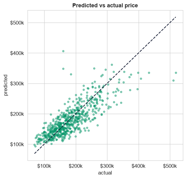
The model's predictions on homes it never saw, plotted against true sale prices; the tight clustering along the diagonal is the honest 0.63 cross-validated fit.
On the log scale, exponentiating a coefficient gives a percentage effect on price. Ranked, the drivers tell a clear story:
Location is king. An otherwise-identical home is worth about 52% more in NorthRidge and 32% more in Somerset than in the baseline neighborhood, but ~10% less in OldTown or Edwards. After location, the kitchen is the biggest controllable lever (about +6% per quality grade), then bedrooms (+6% each) and size (+2% per 100 sqft). Age, extra baths, and central air add nothing once these are in the model. A concrete prediction: an 1,800 sqft, good-kitchen, 3-bed home in CollegeCreek is worth about $226,000 (95% interval $152k–$334k).
Actionable: a renovating owner gets more per dollar from the kitchen than from most additions; an agent must price off neighborhood-specific comps; a buyer can sanity-check any asking price against the model's fair range.
Deploy the model
To turn this into a tool people use: persist the fitted model and the cleaning steps as a
scikit-learn Pipeline; serve it behind a small API (FastAPI/Flask) that
accepts a home's features and returns a price with an interval; score in batch
for nightly re-valuations or on demand for a live widget; add
guardrails (always return the interval, refuse to extrapolate past the training range,
predict on the log scale then exponentiate); and monitor prediction error for drift,
retraining on fresh sales each quarter. The discipline from steps 2–10 is exactly
what keeps a deployed model honest.
Communicate: the Plain-English Write-Up (Step 12)
The last step is the one non-analysts actually read. Here is the whole project with no jargon:
What we found, for a non-statistician
What we did. We took a spreadsheet of 610 past home sales, cleaned it up (removed duplicates and a few unusable rows, fixed typos in the categories, filled in some missing lot sizes, standardized the dates), and built a formula that estimates a home's price from its features.
How good is it? The formula explains about two-thirds of why prices differ (an "R-squared" of 0.65). Tested on homes it had never seen, it held up (0.63), so it is not just memorizing. It reports a price range, not a false-precision single number.
What drives price, in order:
- ✓Neighborhood is the biggest factor, the same house can be worth 50% more or 10% less purely by location.
- ✓Kitchen quality is the biggest thing an owner can change: each grade up is worth about 6%.
- ✓Size adds about 2% per extra 100 sqft; each bedroom about 5.5%.
- ✓Age, extra bathrooms, and air conditioning did not matter once the above were accounted for, a useful, money-saving finding.
The honest caveats. A few luxury homes behave differently, so we used robust error bars and confirmed those homes do not distort the conclusions. The model describes this town's past sales and should be refreshed as the market moves.
Bottom line: location aside, the kitchen is where the money is, and any asking price can be checked against the model's fair-value range.
Run the entire project in Python
The companion notebook is the full 12-step pipeline in code and pictures: it loads the messy CSV, inspects and cleans it (duplicates, categories, dates, missing values), visualizes with histograms, box plots, and a correlation heatmap, log-transforms and encodes, builds the regression, runs the complete diagnostic suite (VIF, residual plots and tests, robust standard errors, Cook's distance, cross-validation), interprets the coefficients as dollars, and closes with a deployment plan and a plain-English write-up. Every table and chart is explained.
View opens the rendered notebook instantly (no setup). Open in Colab runs &
edits it live in your browser. To run locally, install numpy, pandas, scipy,
matplotlib, seaborn, statsmodels, and scikit-learn.
🎓 Key Takeaways
- ✓The method is the skill: define → collect → inspect → clean → visualize → transform → analyze → build → validate → interpret → deploy → communicate. The model is one step of twelve.
- ✓Cleaning dominates real work: duplicates, inconsistent categories, mixed date formats, and two different kinds of missing data (structural "none" vs genuinely unknown) all needed deliberate fixes.
- ✓Transform for the model: a log fixed the skewed price (1.16 → 0.02); ordinal and dummy encoding turned categories into usable features.
- ✓Validate honestly: VIF cleared multicollinearity, but heteroscedasticity was real (robust SEs), a few luxury homes were influential (Cook's distance), and cross-validation (0.63) confirmed no overfit.
- ✓Interpret into decisions: location dominates (NorthRidge +52%), the kitchen is the best controllable lever (+6%/grade), and the answer ends in plain English.
Take It Further
Five ways to extend the case study in the notebook, each exercises a method from earlier chapters:
A different imputation
Impute lot_frontage with a regression on lot area instead of the neighborhood median; does the model change?
Skip the log
Fit the model on raw price instead of log(price) and compare the residual diagnostics.
Add an interaction
Test whether the effect of living area differs by neighborhood (gr_liv_area * C(neighborhood)).
Regularize it
Fit a lasso on the full feature set; does it select the same predictors you kept by hand?
LassoCV on the standardized features (see Regularization & Flexible Models).Price your own home
Build a one-row DataFrame for a house you know and predict its price with an interval.
get_prediction(...).summary_frame(), then exponentiate.All five, worked in a companion notebook
A second notebook, Take It Further, recaps this chapter's model and then works every one of these five extensions with visuals and explanations, a regression imputation, the raw-vs-log comparison, the neighborhood interaction, a lasso, and a price-your-own-home tool, closing with a plain-English summary.
Quiz: Test Yourself
Eight questions on the end-to-end case study. Answer them, hit Check Answers, and keep refining until you score 100%. Your progress is saved, so you can hop back to the chapter and return anytime.
From a dirty CSV to a deployed, explained model. Case Study: Logistic Regression in Action does the same for a yes/no outcome, fitting, reading odds ratios, choosing a threshold, and evaluating a classifier end to end.