Ames predicted a number (price), churn predicted a yes/no. This one predicts a count, whole, non-negative, unbounded, which needs its own model. Fit a straight line to daily rentals and it will happily forecast negative demand; the right tool is Poisson regression, and it has one famous failure to watch.
Everything from steps 1–7 is the familiar pipeline. The new content lands at steps 8–9: choose a Poisson family, then discover the daily counts are wildly overdispersed and switch to a negative binomial.
The 12-Step Method
The same repeatable loop, now applied to a count outcome. The companion notebook runs all twelve steps in code; the sections below narrate the story with the key numbers and pictures.
Two years of daily records: date, season,
weather, temp_c, humidity, windspeed, workingday,
holiday, and the target rentals (a daily count).
Define, Collect, Inspect, Clean (Steps 1–4)
Define the objective
Predict the daily rental count and identify its drivers, so operations can pre-position bikes, schedule staff, and time maintenance. Because rentals are counts, ordinary linear regression is wrong (it can predict negative demand); the right family is Poisson.
Collect the data
A CSV pull from the bike-system database. As always, other sources (SQL, an API, a spreadsheet) would use the same one-line pandas readers, then land in a DataFrame.
Inspect the data
info() and value_counts() reveal the mess: season and weather
in mixed case, workingday as 0/1 and Yes/No, three date formats, duplicate days, missing weather
readings, and a few rows with no rentals.
Clean the data
| Problem | Detail | Fix |
|---|---|---|
| Missing target | 5 rows with no rentals | drop |
| Duplicate days | 14 repeated dates | deduplicate |
| Messy categories | season ×12, weather ×8, workingday 0/1 + Yes/No | normalize case, map to one scheme |
| Three date formats | date | pd.to_datetime(format="mixed"), then engineer month & weekend |
| Missing weather | humidity 18, windspeed 9 | impute the median |
After cleaning, 726 days remain with no missing modeling values, and we have engineered
month and is_weekend from the parsed dates.
Visualize, Transform, Analyze (Steps 5–7)
Visualize the data
Demand tracks the weather and the temperature. Average rentals fall from about 1,700 on clear days to under 400 in heavy rain, and rise with temperature (the scatter climbs, then flattens in the heat). The count distribution is right-skewed, and its spread grows with its level, the first hint of trouble.
Transform features
We engineer calendar features (month, weekend) from the date, enter weather and season as
dummy variables, and add a squared temperature term to capture
the rise-then-flatten shape. The outcome is a count, so the model family is Poisson with a log link.
Analyze patterns
Quantifying the hint: the daily rentals have a variance-to-mean ratio in the hundreds, when a Poisson model assumes it is about 1. That is overdispersion, and step 9 must deal with it.
Build and Validate (Steps 8–9)
Build the model
A Poisson GLM of rentals on temperature (and its square), humidity, windspeed, weather, season,
working day, and holiday. It fits well, but its Pearson chi-square / df is about 255 (it should be
near 1), the overdispersion alarm.
Validate the model
Bin the data and the variance sits far above the mean, Poisson's core assumption is badly violated:
The remedy is the negative binomial, which adds a dispersion parameter so variance can exceed the mean. It is a spectacular improvement here, the AIC drops from about 183,000 to 11,000. VIFs are ~1 (no multicollinearity), and the negative-binomial forecast tracks actual demand closely (pseudo-R² ≈ 0.66):
Same rate ratios as the Poisson fit, but now with honest standard errors. This is the count analog of the log transform in the house-price study: diagnose the violation, switch to the right model, re-check.
Interpret and Deploy (Steps 10–11)
Interpret the results
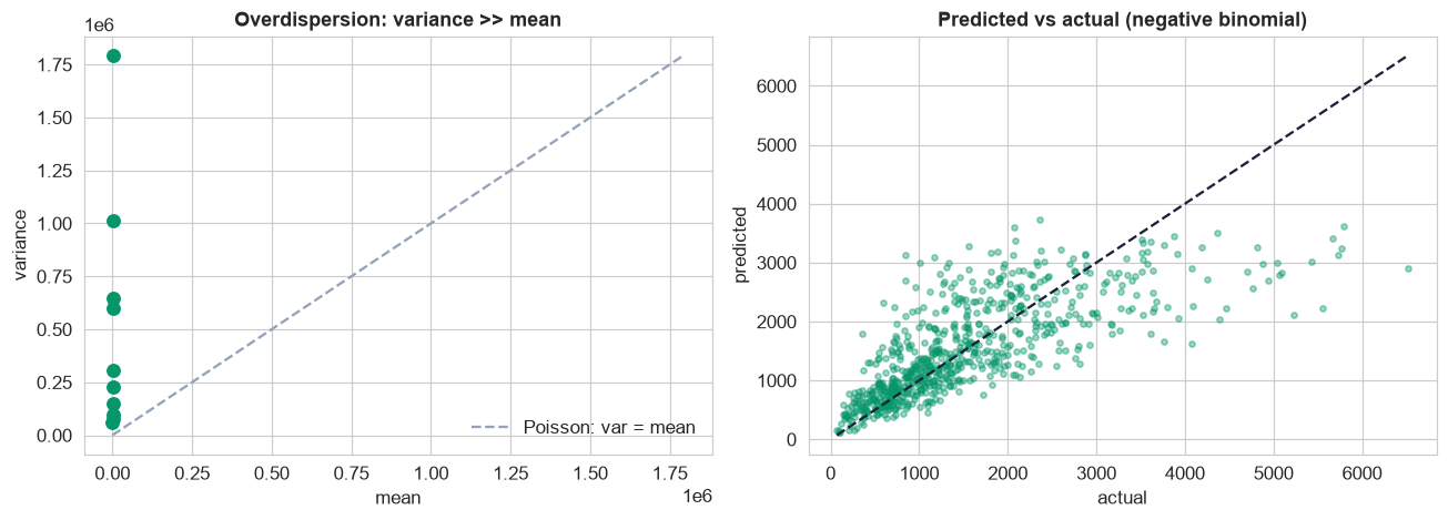
The variance-versus-mean overdispersion check (why negative binomial beats plain Poisson here) alongside the fitted demand forecast.
Exponentiating each coefficient gives a rate ratio, the multiplier on expected demand:
Weather rules demand. A heavy-rain day sees only ~25% of clear-day rentals, light rain about half. Warmth helps (+33% for every 5°C), working days run ~10% busier than weekends, and holidays ~40% quieter. A concrete forecast: a warm, clear working day predicts about 3,000 rentals.
Actionable: scale bikes and staff down on forecast rain and cold, up on warm clear working days, and treat holidays like weekends. The forecast feeds straight into the next day's rebalancing plan.
Deploy the model
Persist the model and cleaning as one pipeline; score daily by feeding tomorrow's weather forecast plus the calendar to get a predicted count with a range; feed it into bike rebalancing, staffing, and maintenance planning; monitor forecast error and retrain as ridership grows. Guardrail: report the interval and do not extrapolate to weather far outside the training range.
Communicate: the Plain-English Write-Up (Step 12)
For the operations manager
What we did. We took two years of daily rental records, cleaned them (removed duplicate days and a few unusable rows, fixed inconsistent labels, filled a handful of missing weather readings, standardized the dates), and built a formula that predicts how many bikes will be rented on a given day.
How good is it? It explains about two-thirds of the day-to-day swing in demand and tracks actual rentals closely, reporting a sensible range rather than a single number.
What drives demand:
- ✓Weather above all, a rainy day can cut rentals by up to 75%.
- ✓Temperature, warmer days are busier (about +33% per 5°C).
- ✓The calendar, working days beat weekends; holidays are quiet.
A note on method. Daily counts bounce around far more than a simple model expects, so we used one built for that (a "negative binomial"), which makes the forecast's confidence honest.
In practice: let tomorrow's weather forecast set tomorrow's bike plan.
Run the entire forecast project in Python
The companion notebook is the full 12-step pipeline: it loads and cleans the messy daily export (dates, categories, missing weather), visualizes demand and its seasonal rhythm, engineers calendar features, fits Poisson then negative-binomial regression, diagnoses overdispersion (variance-vs-mean, Pearson chi-square), reads rate ratios, and forecasts a day, with every table and chart explained.
View opens the rendered notebook instantly.
Open in Colab runs it live. To run locally, install numpy, pandas,
matplotlib, seaborn, statsmodels, and scikit-learn.
🎓 Key Takeaways
- ✓Counts need a count model: Poisson regression (log link) predicts a non-negative rate; ordinary regression can predict negative demand.
- ✓Coefficients exponentiate to rate ratios: heavy rain ×0.25, +5°C ×1.33, working day ×1.10.
- ✓Overdispersion is the count-model pitfall: the variance-to-mean ratio and Pearson chi-square / df flagged it (in the hundreds).
- ✓The negative binomial is the fix: it let variance exceed the mean and cut the AIC from ~183,000 to ~11,000, honest error bars, same rate ratios.
- ✓Same 12-step method as the other case studies, only the model family (and its diagnostic) changed for a count outcome.
Take It Further
Five ways to extend the forecast in the notebook:
Poisson vs negative binomial, quantified
Compare the two models' standard errors on the weather coefficients to see how much Poisson understated them.
.bse from each fit.Does temperature really curve?
Refit without the squared temperature term and compare AIC; is the curvature worth keeping?
Cross-validate the forecast
Use 5-fold CV to estimate out-of-sample accuracy and confirm the model is not overfit.
PoissonRegressor with cross_val_score.Weekend vs weekday profiles
Test whether weather hurts weekend demand more than weekday demand (an interaction).
C(weather) * is_weekend.Forecast a week ahead
Build a 7-row DataFrame from a weather forecast and predict each day's demand with a range.
get_prediction(...).summary_frame().All five, worked in a companion notebook
A second notebook, Take It Further, recaps this chapter's model and then works every one of these five extensions with visuals and explanations, the Poisson-vs-NB standard errors, the temperature curve, cross-validation, a weekend-weather interaction, and a week-ahead forecast, closing with a plain-English summary.
Quiz: Test Yourself
Eight questions on the count-regression case study. Answer them, hit Check Answers, and keep refining until you score 100%. Your progress is saved, so you can hop back to the chapter and return anytime.
You have now modeled a number, a yes/no, and a count, end to end. Predicting Medical Charges tackles the last frontier of this Part: a regression with many predictors, where regularization picks the signal from the noise.