Part XXIX was about designing your way to a causal answer. This part is about the craft of the model itself, and it starts with the decision that regression makes easiest to get wrong: which variables belong on the right-hand side.
- Setting
- A company's HR system: 3,600 employee records with gender, age, years of experience, education, department, job level, most recent performance rating and annual salary.
- The question
- Are women paid less than men at this company, and if so, by how much?
- Why it matters
- The answer goes into a regulatory filing and possibly into litigation. It will be read by people who want a single number, and quoted by people who want a small one.
- What we do
- Model log pay, add controls one at a time so every step is visible, measure the collinearity among the career variables and show exactly what it does, then stop before the most powerful control and ask whether the company assigns it equally before deciding whether it belongs in the model at all.
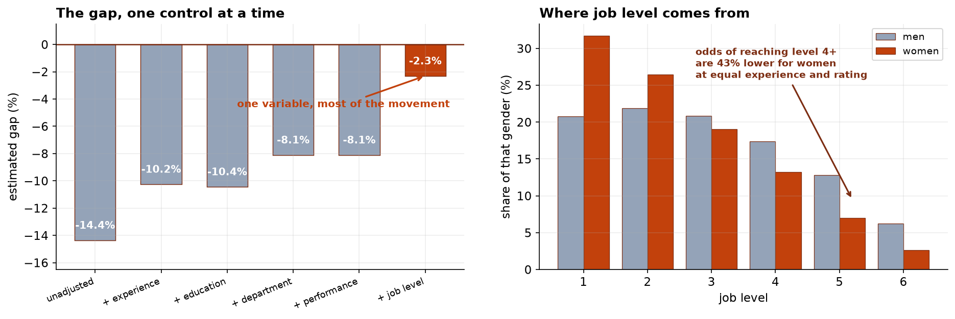
Unadjusted, women earn 14.4 percent less. Experience, education and department take that to 8.1 percent. Job level alone takes it to 2.3 percent. But at equal experience, education, performance and department, women's odds of reaching level 4 or above are 43 percent lower, so job level is carrying the very thing the review is looking for.
Two Questions, Not One
The most common failure in a pay equity review is producing a single number. There are two, they mean different things, and either one on its own is an answer to a question somebody else asked.
| The unadjusted question | The adjusted question | |
|---|---|---|
| Asks | What do women in this company earn, against what men earn? | Among people doing similar work with similar backgrounds, what is the difference? |
| Describes | The workforce as it actually is | How individuals are paid within a grade |
| Used for | Reporting, and asking why the distribution looks like that | Pay-setting policy, and individual review |
| Fails when | Quoted as evidence about individual pay decisions | Quoted as the company's pay gap |
Both get reported. Neither is "the" pay gap, and the analysis plan for this review said so in writing before the salary file was opened, alongside one further commitment: we will not control for a variable the company itself assigns unless we have checked whether it is assigned equally.
Cleaning, and One Decision Worth Defending
| Step | Records | What happened |
|---|---|---|
| HRIS export | 3,648 | The extract ran twice |
| After deduplication | 3,600 | One row per employee |
| Salaries of zero voided | 3,591 | Nine payroll errors, not nine unpaid employees |
| Experience sentinels voided | 3,569 | Twenty-two records carried −1, which is not a tenure |
| Missing performance ratings | 69 kept | Filled with the median and flagged with an indicator |
That last row is the decision worth defending. Dropping the sixty-nine people with no review on file would have
silently changed who the study is about, and people without a recent review are not a random sixty-nine. Filling
the rating with the median and adding a perf_missing indicator keeps them in the analysis and keeps
the fill visible to the model, so the coefficient on the indicator can tell you whether those employees differ.
The Specification Ladder
The outcome is the log of salary, so coefficients read as approximate percentage differences. Controls go in one at a time, because anyone can produce a small number by adding enough variables and the honest presentation is to show the number moving.
| Specification | Estimated gap | 95% interval | R² |
|---|---|---|---|
| Unadjusted | −14.36% | — | — |
| + experience | −10.25% | [−11.92%, −8.55%] | 0.261 |
| + education | −10.44% | [−12.05%, −8.80%] | 0.309 |
| + department | −8.10% | [−9.64%, −6.54%] | 0.415 |
| + performance | −8.10% | [−9.58%, −6.61%] | 0.468 |
| + job level | −2.31% | [−3.08%, −1.53%] | 0.875 |
Read the last row against the one above it. Experience, education, department and performance between them take the gap from 14.4 percent to 8.1. Job level alone takes it from 8.1 to 2.3, and the R-squared leaps from 0.47 to 0.88. One variable is doing more work than all the others combined, and it happens to be the only variable on the list that the company assigns to people.
Notice also that performance changed nothing at all. Men and women in this workforce are rated the same, which is worth reporting: it removes one common explanation before anybody offers it.
Collinearity, and What It Actually Does
Age, experience and job level all measure roughly one underlying thing: how far into a career somebody is. Age and experience correlate at 0.829 here, which is unremarkable for a real workforce and enough to matter.
A VIF of 3.4 violates nothing. The thresholds people quote, 5 or 10, are conventions rather than rules, and the practical consequence is easier to see by looking directly at what happens when both variables go in.
| Model | Experience | Age | The gender coefficient |
|---|---|---|---|
| Experience only | +0.01060 (SE 0.00043) | — | −0.0234 (SE 0.0040) |
| Age only | — | +0.00705 (SE 0.00036) | −0.0273 (SE 0.0041) |
| Both | +0.01013 (SE 0.00072) | +0.00048, p = 0.41 | −0.0234 (SE 0.0040) |
Two things happen, and only one of them is what people expect. Putting both in inflates the standard error on experience by about two thirds, and leaves age with nothing left to explain. What does not happen is any movement in the coefficient we care about: the gender gap sits at −0.0234 either way.
Collinearity between two controls damages the estimates of those controls and leaves the rest of the model alone. If neither age nor experience is the quantity of interest, high VIFs among them are a reason to simplify for interpretability, not a threat to the finding. Panic about multicollinearity is usually misdirected: the question is never "is the VIF above 5", it is "is the variable whose standard error just doubled the one I am trying to measure".
We keep experience and drop age, because experience is what the company's pay policy claims to reward, and a coefficient the reader can map onto a policy is worth more than one they cannot.
The Control That Should Not Be Added Without an Argument
Job level took the gap from 8.1 percent to 2.3. Before accepting that as the adjusted answer, ask what job level is. It is not a fact about an employee, like their education. It is a decision the company made about them.
If women are promoted more slowly than their experience and performance warrant, then job level is partly a result of unequal treatment. Controlling for it asks whether people are paid fairly once they have arrived at a grade, and treats how they arrived as fixed. That is a legitimate question. It is not the same question, and the regression output looks identical whichever it is answering.
So the plan required checking. At equal experience, education, performance rating and department, what are the odds of an employee sitting at level 4 or above?
This is the finding the adjusted model deletes. Women are 43 percent less likely to sit at senior grades than men who look identical on everything the company says it promotes on. A report giving only the 2.3 percent figure would be arithmetically correct and would leave the mechanism producing most of the gap entirely unmentioned.
An Average That Describes Nobody
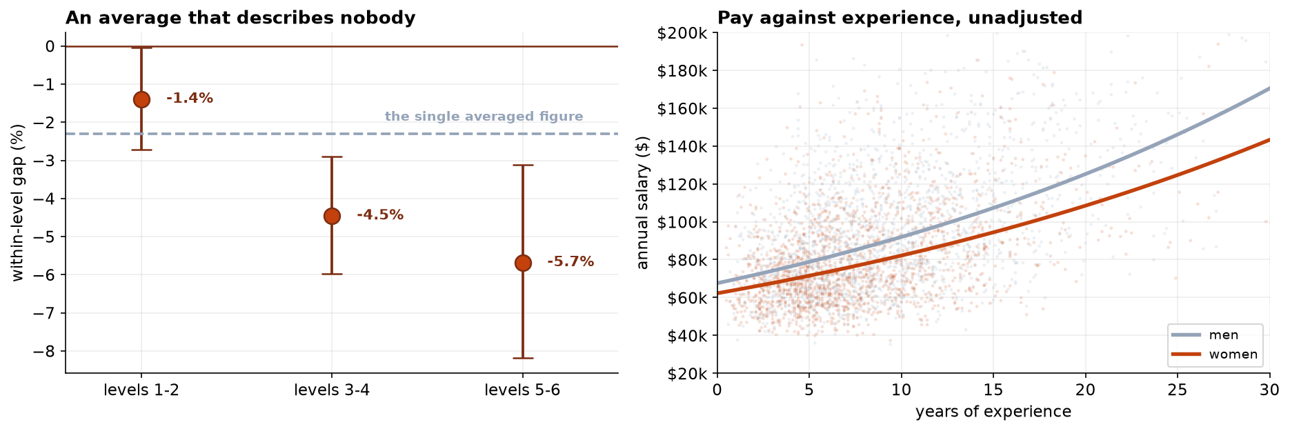
The 2.3 percent is itself an average across the whole company, and the plan asked in advance whether the within-level gap is the same at every level. It is not.
| Job levels | Within-level gap | Against the single average of −2.3% |
|---|---|---|
| 1 to 2 | −1.39% | The average overstates it by two thirds |
| 3 to 4 | −4.45% | Nearly twice the average |
| 5 to 6 | −5.68% | Two and a half times the average |
The test that the gap is constant across levels returns p = 0.0012, so that pattern is not noise. Quoting 2.3 percent to a woman at level 5 would understate her position by more than half, and quoting it to a woman at level 1 would overstate hers. An average is a summary of a distribution, and it is only a good summary when the distribution has one mode.
Diagnostics, and How to Read a Screening Rule
All three pass, and the influence line needs reading carefully rather than quoting. One hundred and seventy observations exceed the familiar 4/n cutoff, which sounds alarming and is not. 4/n is a screening rule, not a threshold for concern: in a sample of 3,569 it flags roughly the top few percent by construction, whatever the data look like. The number that matters is the magnitude, and the largest Cook's distance here is 0.007 against conventional cause for concern at 0.5. No single employee is moving this model.
Chapter 187 is about what to do when these checks fail, which they do more often than published papers suggest. Here they pass, and verifying that is worth the four lines it costs.
What to Actually Report
Three numbers, each with a sentence saying what it means. Not one number, and not three numbers offered as alternatives for the reader to choose between.
| Report | Figure | The sentence that has to go with it |
|---|---|---|
| The workforce gap | −14.4% | What women at this company earn against what men earn. It reflects who holds which jobs, not what any individual is paid for the same work. |
| The promotion gap | Odds 0.569 | At equal experience, education, performance and department, women are 43 percent less likely to hold a senior grade. This is where most of the workforce gap comes from. |
| The within-grade gap | −1.4% to −5.7% | At the same grade, women are paid slightly less, and the difference grows with seniority. |
Presented that way, the company has a clear picture and a clear place to look. Presented as "our adjusted pay gap is 2.3 percent", it has a defensible-sounding number and no idea where its problem is.
What to Watch
- ✓Never control for a variable the organization assigns without checking how it is assigned. Job level took the gap from 8.1 percent to 2.3. That is either the right adjustment or the erasure of the finding, and only the promotion model can tell you which.
- ✓Show the ladder. Anyone can reach a small number by adding variables, and the sequence is the first thing an opposing expert will reconstruct. Publishing it yourself costs nothing and removes the accusation.
- ✓Collinearity is a problem for the collinear variables. Check whether the standard error that inflated belongs to the coefficient you are reporting. Here it did not, so the VIFs were a formatting decision rather than a threat.
- ✓Test the interaction before averaging. A gap of 2.3 percent that runs from 1.4 to 5.7 across the company describes nobody in it.
- ✓A coefficient is not a finding about any individual. It is evidence about a pattern, and it tells you where to look rather than what any one person is owed. Individual cases need individual review.
- ✓Watch what a small adjusted figure gets used for. It is easy to quote as a clean bill of health, and what it actually says is narrower: within a grade, pay is nearly equal. Whether people reach that grade equally is a separate and less comfortable question.
- ✓Gender here is a recorded binary field. That is what the HR system holds. It excludes non-binary employees and anyone whose record is wrong, and the analysis inherits both limitations rather than solving them.
Specification Choices in Data Science & AI
| Where it appears | The same decision, in a different costume |
|---|---|
| Feature selection for models | Adding a feature that the model's own past decisions produced, so the model learns to reproduce them |
| Fairness auditing | Deciding which attributes to condition on, where conditioning on a proxy for the protected attribute hides the disparity |
| Credit and hiring models | Job title, seniority or prior salary as features, each of which can carry historic discrimination forward |
| Uplift and marketing models | Controlling for engagement that the campaign itself produced |
| Any regression with an ML pipeline | Automated feature selection makes the mediator decision silently and at scale, with no analyst to argue with |
The mediator problem has a precise name in the causal literature: conditioning on a post-treatment variable, treated formally by Rosenbaum in 1984 and now standard in Pearl's graphical framework, where the rule is simply that you do not condition on a descendant of the exposure. The decomposition into direct and indirect effects is the subject of causal mediation analysis, which gives estimators for exactly the two paths this chapter separates by hand. On the applied side, the Oaxaca-Blinder decomposition is the economist's standard tool for splitting a gap into an explained and an unexplained part, and it inherits the same difficulty: what counts as explained depends entirely on which variables you were willing to put in.
The full project, step by step
The companion notebook reads the plan before the salary file, cleans the export and keeps the employees with no review on file, builds the specification ladder with an interval at every rung, shows what collinearity does to the standard errors and what it leaves alone, fits the promotion model that job level was concealing, tests the interaction across levels, and closes with the diagnostics and how to read a screening rule.
The dataset
(capstone-pay-equity-review.xlsx) holds 3,648 HR records with their duplicate export, payroll
zeros, experience sentinels and missing reviews intact, the analysis plan agreed before the salary file was
opened, and the parameters that generated the data so every estimate can be checked. Two written reports
accompany it: a plain-language brief for the HR director who has to act on it, and a
technical report written to survive an opposing expert.
🎓 Key Takeaways
- ✓A pay gap has two honest answers. The workforce gap is 14.4 percent and the within-grade gap is 2.3, and each is the wrong answer to the other's question.
- ✓Adjusting for a mediator deletes the effect. Job level took the gap from 8.1 to 2.3 because women are 43 percent less likely to hold senior grades at equal experience and rating.
- ✓Collinearity hurts the collinear variables. Age and experience together inflated experience's SE by two thirds and left the gender coefficient at −0.0234 exactly.
- ✓Test the interaction before averaging. The within-level gap runs from −1.4 percent at junior grades to −5.7 at senior ones, p = 0.0012.
- ✓4/n is a screening rule, not a verdict. A hundred and seventy points cleared it and the largest Cook's distance was 0.007.